A short while ago, Santa Claus came to me for a short visit to drink a cup of tea together. That was very pleasant, but I had the idea that there was something more, knowing that he is always busy, especially these days. After some time, he came forward and said that the elves had found my distribution GnomeTools and were eager to use it. It looks so promising. However, they had problems finding any documentation about it. I had to admit that there was still a lot missing. My excuse was that the package needed a lot more classes and might also change here and there. Santa Claus said that that shouldn’t be a problem as long as I keep the version below 1 ;-). Santa said that he would like to see some examples so that his elves could do something with the classes.
Ok, here we go then …
Very short example
For the people working a lot with scripting languages, it would be nice to show some information in a kind of message dialog. This next example will show a simple way to do just that. The dialog window will disappear after pressing the OK button.
use GnomeTools::Gtk::MessageDialog;
myStr$message=Q:q:to/EOM/; I would heavely recommend continuing using the Raku language whatever your plans are in the near or distant future, because it will bring you fortune and happyness! EOM
my GnomeTools::Gtk::MessageDialog $message-dialog; $message-dialog.=new(:$message);
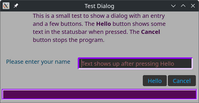
And the result …
A Dialog
A more elaborate example is a dialog window that shows more than just text. We start by getting the necessary ingredients and a simple class with callback methods. These methods are called from the native routines. The method reads the text entry and copies this string into the status field. Both fields are in the dialog, which we will see later.
use GnomeTools::Gtk::Dialog;
use Gnome::Gtk4::Label:api<2>; use Gnome::Gtk4::Entry:api<2>;
Then we create a header text for the dialog and a text entry field with a placeholder text instructing you what to do.
After that, the dialog is created with a title and a header. A statusbar is added below the button row.
In this dialog window, we add content. It always consists of a text line on the left and a widget to its right. In this case, a text entry. You can add as many rows as you like.
Then, buttons are added. One ‘Help’ button which, when clicked, calls the say-hello() routine defined earlier. The other is to tear down the dialog window.
myStr$dialog-header=Q:a:to/EOHEADER/; This is a small test to show a dialog with an entry and a few buttons. The <b>Hello</b> button shows some text in the statusbar when pressed. The <b>Cancel</b> button stops the program. EOHEADER
withmy Gnome::Gtk4::Entry $entry.= new-entry { .set-placeholder-text( 'Text shows up after pressing Hello' ); .set-size-request( 400, -1); }
my GnomeTools::Gtk::Theming $theme.=new(:$css-text); $theme.add-css-class( $entry,'dialog-entry');
Nice, isn’t it! The CSS classes dialog-tool, dialog-header, dialog-content, and dialog-button are defined in the GnomeTools::Gtk::Dialog class. The CSS class statusbar-tool is defined in the GnomeTools::Gtk::Statusbar class. In the program, we added the class dialog-entry. Note, however, the CSS used by Gnome is not exactly the same as one might be used to, You can find good information here.
Note that the call to .show-dialog() does not return until the cancel button is clicked, which destroys the dialog window. So, for the shell scripting elves, we could add a line just to the end, like so;
.show-dialog; }
say$entry.get-text
This gives us the possibility to return information into a shell script. For example, when this program is stored in file xt/dialog.rakutest;
echo Hello `raku xt/dialog.rakutest`
Installing and other info
You can install this distribution with zef
> zef install GnomeTools
Reference information on Gnome::* modules can be found here.
First, let’s import all the libraries we need – you’ll need to use zef to install what you don’t have:
use PDF::API6;
use PDF::Content::Color :rgb;
use PDF::Annot::Link;
use PDF::Destination :Fit;
use PDF::Content::FontObj;
use Date::Names;
We’re going to do a lot of hardcoding towards A4, and just work for 2026 in this case so developing this further will certainly involve more variables! But create a pdf, set it to ‘A4’ and create our start date which has to be the first of the fist due to all the counting I’m doing on my hands and toes
my $pdf = PDF::API6.new();
$pdf.media-box = 'A4';
my $start_date = Date.new(2026, 1, 1);
my PDF::Page $page;
my PDF::Content::FontObj $font = $pdf.core-font('Helvetica-Bold');
We’re also going to add an index to the pdf, so let’s set up an array for that and a reusable title variable
my $bookmarks = [];
my $bookmark-title = '';
We’re going to create a pdf with all the pages we need. At first I was going to create page content as I went, but for linking to other pages, the page must exist.
So here we create a big, blank pdf that has 12 pages at the front for the months of the year and 365 pages following for every day of the year. And by using days-in-year we’ll be ready when we update to do years involving leap years.
for 1..(12 + $start_date.days-in-year) {
    $page = $pdf.add-page;
};
This is a handy sub taken from the very full documentation for PDF::Api which will make our links tidier, and you’ll see used in the following loop
sub dest(|c) { :Dest($pdf.destination(|c)) }
Let’s start filling the pages!
We’ll do the first 12 pages will are our months of 2026. Use the handy raku loop shortcut of creating our $month variable. And we know our months are pages 1-12 of our blank pdf.
We want a variable we can change that starts as the start date, but we don’t want to change the actual start date. And also we’ll be using nice date names as we’ll be writing dates on our PDF for real people – me!
It’s worth mentioning that the co-ordinates on pdfs are (x, y) – with x being how far from the left and y being how far from the bottom you are plotting.
So (0,0) on a pdf is the bottom left.
my $current_date = $start_date;
my $nice_date_name = Date::Names.new;

for 1..12 ->$month  {
    $page = $pdf.page($month); # Access the first 12 pages in turn
    my $text = ($nice_date_name.mon($current_date.month)); # Set text ie 'January', 'February'...
    $bookmark-title = $nice_date_name.mon($current_date.month); # Also remember our document outline
    $bookmarks.push( %(( :Title($bookmark-title)), dest(:page($page))));


    $page.gfx.text: {
        .font = $font, 20; # We set our font earlier as a variable, but hardcoding the size here
        .text-position = 250, 800; # And we're targeting the top middle of the A4 pdf page
        .say($text); # Boom! We've written on our page, but not done yet...
    }
So, one page at a time we’re writing the month at the top of the pdf page – all in memory so far. But it might be nice to decorate a bit further.
We’ll continue the loop by putting in the day number of the month, with the day and a helpful horizontal line for writing notes on.
But we’re going to make that link to the page for that particular day too, so we can make overview notes here, but jump to the full page for more detailed notes.
(It should also be noted that I tried this in the kindle app on Android and the links didn’t work, but they worked fine on Samsung notes and my pdf app on my PC – think this is actually a limitation of kindle rather than me.)
my $height = 750; # So, this is nearish the top in 'points' on an A4 pdf
for 1..$current_date.days-in-month ->$day { # days-in-month - built into raku and very handy!
    my $text = $day ~ " (" ~ $nice_date_name.dow($current_date.day-of-week, 3) ~ ")";
    # So our text will look like '1 (Mon)', '2 (Tue)' or whatever…
    $page.gfx.text: {
    .font = $font, 20; # We're creating text as before
    # We're going to draw a line under this text, so a little positional adjustment
    .text-position = 20, $height + 2;
    # This text is going to be a link rather than plain text!
    my PDF::Annot::Link $link = $pdf.annotation(
    :border-style({:width(0)}),
    :page($page),
    :text($text),
    # Using our sub for the intricacies, let's make the target the main page for this date
    # But adjusting it by 12 because our first 12 pages in the pdf are the months of the year.
    # And this is why we created the whole pdf at the beginning - linking to a page that doesn't
    # exist will break.
    |dest(:page( $current_date.day-of-year + 12 )),
    );
};
So we’ve done two types of text – plain text and linking text – now lets draw our lines under the date we just wrote.
    $page.gfx.paint: :fill, :stroke, { # Painting rather than texting
        .StrokeColor = rgb(.211, .211, .211);
        .LineWidth = 2.5;
        .current-point = (20, $height); # Lines go from somewhere...
        .LineTo(575, $height); # ...to somewhere
    };

    $height = $height - 24; # We want our next date and the line to be lower
    $current_date++; # Add we're in a loop for this month so let's go to the next day
};
};
So, we’ve now gone through our first 12 pages, putting the month name at the top and writing all the days vertically down the page, with a horizontal line for writing notes on. All very profesh!
Next we want to go through the daily pages of the journal. For these we’re just going to create a blank page with the day’s date on the top.
Obviously, there’s scope to go through the line drawing again, or perhaps look into drawing a border with a rectangle? Or maybe print a random quotation from somewhere on it, or use a pdf template you’ve drawn in some other app and just want to print the days date on.
We’re doing this for the joy of being able to personalise our digital stationary – you can of course spend not very much money buying something very nice off Etsy, but it’s nice to have so many options.
$current_date = $start_date; # Let's remember to reset to the first day of the year

for 13..($start_date.days-in-year + 12) ->$day  { # Adjust for our 12 monthly pages at the beginning
    $page = $pdf.page($day);
    my $text = (
          $nice_date_name.dow($current_date.day-of-week)
        ~ ' ' ~
        $current_date.day
        ~ ' ' ~
        $nice_date_name.mon($current_date.month)
    ); # So, 'Monday 12 January', 'Friday 29 May' or whatever

    # Remembering we're doing our outline...
    $bookmark-title = $nice_date_name.dow($current_date.day-of-week) ~ ' ' ~ $current_date.day ~ ' ' ~ $nice_date_name.mon($current_date.month);
    $bookmarks.push( %(( :Title($bookmark-title)), dest(:page($page))));

    $page.gfx.text: {
        .font = $font, 20;
        .text-position = 200, 800;
        .text-position = 200, 800;
        my PDF::Annot::Link $link = $pdf.annotation(
            :border-style({:width(0)}),
            :page($page),
            :text($text),
            # So we're creating a link as before and we want to link to one of the first 12 pages
            # that corresponds to the month we're in
            |dest(:page($current_date.month)),
        );
    };

    $current_date++; # Move onto the next day
};
Then the last things we need to do are save our outline to the pdf and save our pdf for wrapping up and putting under the digital tree.
And we are ready to be organised next year with a PDF journal that has handy linking and lots of opportunities for improvement. Perhaps it might be nice to add more pages into the daily part – todo, to sketch, notes. Or perhaps another section that contains all the months on one page so you can jump from there to the individual months?
But there’s plenty of scope for making it more flexible to accept a year and a page size at the very least, but for now – I have what I need.
“Advent is here”, the buzz was all around, the elves were getting nervy and the reindeer pawed the ground.
Rudolph (for it was he) stood in quiet contemplation as the elves increased their pace and the din grew ever louder. As we every other Christmas, he was wondering how to get the job done – checking and rechecking all the flight system and navigation data.
He cracked open his laptop – Linux, of course, for that is the leading nordic OS – and opened a Command Line Terminal session. Being a Raku fan of old, he had caught wind of a new feature in the App::Crag model -> inbuilt support for LLM::DWIM (that famous LLM CLI module by the awesome Brian Duggan) and his hooves started to clack away on the keys.
Light Speed
The first challenge was to work out the total distance to travel on Christmas Day and then to know what speed Santa’s slight would need to average in order to get around the entire Earth in just 24 hours.
Click fullscreen to enlarge text…
Wowee – 3.5% of the speed of light (c), eh?
Also – Rudolph was quite impressed with the new built in App::Crag LLM features … boy those Raku guys knew how to jump on a bandwagon. A command line calculator that can source the value of just about anything right there, convert to units of measurement for dimensional analysis and assign to temporary variables so that unit math is comprehensible and that you can backtrack and amend any mistakes or changes along the way. No need to look up planetary stats, physics constants … or even do a text LLM query for advice on formulae.
[Kids – do not even think about using App::Crag to cheat on your end of term exams]
Lorentz Contraction
And that made him wonder about the Lorentz contraction, would they still be ablt to fir all the gifts into the sleigh? [editor note: Rudolph is genius level for a reindeer, ok!]
Amazing – the sleigh would only contract by 7.4214mm – just a sliver and space for gifts aplenty.
Rudolph nodded sagely and lit his MeerSchaum, it would be alright on the night after all.
Rudolph’s calm and cozy, no rush, no need to roam— he’s happily puffing his meerschaum pipe by the stables’ frosty dome.
oh, but what about the relativistic time dilation???!!!
Find out if Christmas can go on after all in the next thrilling instalment…
~librasteve
Credits
Some of the App::Crag features in play tonight were:
?<some random LLM query>
^<25 mph> – a standard crag unit
?^<speed of a diving swallow in mph> – put them together to get units
25km – a shortcut if you have simple SI prefixes and units
$answer = 42s – crag is just vanilla Raku with no strict applied
Checkout the crag-of-the-day for more – but beware, this is kinda strangely addictive.
This document provides an overview of Raku packages, as well as related documents and presentations, for doing Data Science using Raku.
This simple mnemonic can be utilized for what Data Science (DS) is while this document is being read:
Data Science = Programming + Statistics + Curiosity
Remark: By definition, anytime we deal with data we do Statistics.
We are mostly interested in DS workflows — the Raku facilitation of using Large Language Models (LLMs) is seen here as:
An (excellent) supplement to standard, non-LLM DS workflows facilitation
A device to use — and solve — Unsupervised Machine Learning (ML) tasks
(And because of our strong curiosity drive, we are completely not shy using LLMs to do DS.)
What is needed to do Data Science?
Here is a wordier and almost technical definition of DS:
Data Science is the process of exploring and summarizing data, uncovering hidden patterns, building predictive models, and creating clear visualizations to reveal insights. It is analytical work analysts, researchers, or scientists would do over raw data in order to understand it and utilize those insights.
Remark: “Utilize insights” would mean “machine learning” to many.
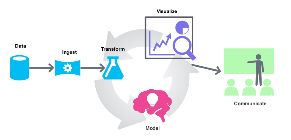
This is the general workflow (or loop) for doing DS:
Assume you have a general purpose language which is very good at dealing with text and a package ecosystem with a well maintained part dedicated to doing various Web development tasks and workflows. (I.e. trying to re-live Perl’s glory days.) What new components the ecosystem of that programming language has to be endowed with in order to make it useful for doing DS?
The list below gives such components. They are ranked by importance (most important first), but all are important — i.e. each is “un-skippable” or indispensable.
Data import and export
Data wrangling facilitation
Statistics for data exploration
Machine Learning algorithms (both unsupervised and supervised)
Data visualization facilitation
Interactive computing environment(s)
Literate programming
Additional, really nice to have, but not indispensable components are:
Data generation and retrieval
Interfaces to other programming languages and ecosystems
Interactive interfaces to parameterized workflows (i.e. dashboards)
LLM utilization facilitation
Just an overview of packages
This document contains overlapping lists of Raku packages that are used for performing various types of workflows in DS and related utilization of LLMs.
Remark:The original version of this document, written a year ago, had mostly the purpose of proclaiming (and showing off) Raku’s tooling for DS, ML, and LLMs.
At least half a dozen packages for performing ML or data wrangling in Raku have not been included for three reasons:
Those packages cannot be installed.
Mostly, because of external (third party) dependencies.
When tried or experimented with, the packages do not provide faithful or complete results.
I.e. precision and recall are not good.
The functionalities in those packages are two awkward to use in computational workflows.
It is understandable to have ecosystem packages with incomplete or narrow development state.
But many of those packages are permanently in those states.
Additionally, the authors have not shown or documented how the functionalities are used in longer computational chains or real-world use cases.
The examples given below are only for illustration purposes, and by no mean exhaustive. We refer to related blog posts, videos, and package READMEs for more details.
Just look (or maybe, download) the mind map in the next section.
And the section “Machine Learning & Statistics“.
Just browse or read the summary list in the next section and skim over the rest of the sections.
Read all sections and read or browse the linked articles and notebooks.
Actually, it is assumed that many readers would read one random section of this document, hence, most of the sections are mostly self-contained.
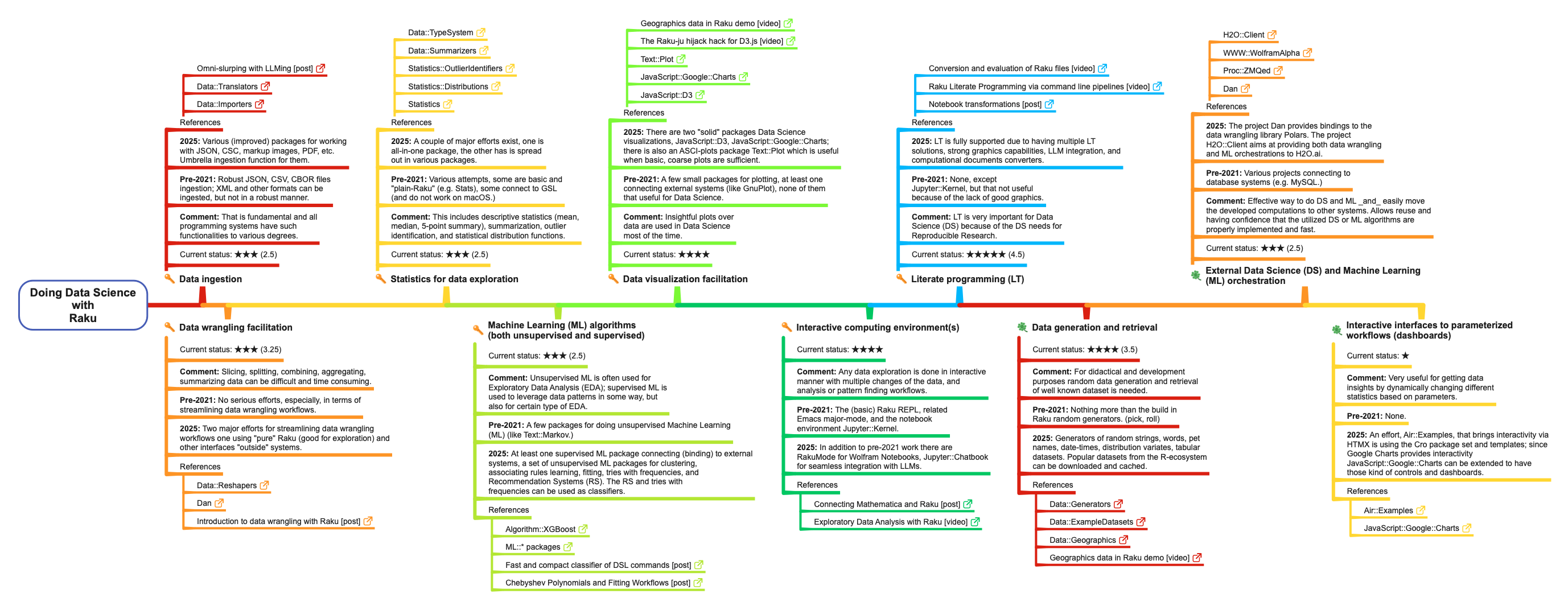
Summary of Data Science components and status in Raku
The list below summarizes how Raku covers the Data Science (DS) components listed above. Each component-item has sub-items for its “previous” state (pre-2021), current state (2025), essential-or-not mark, current state 1-to-5 star rating, and references. There are also corresponding table and mind-map.
Remark: Current-state star ratings are, of course, subjective. But I do compare Raku’s DS ecosystem with those of Python, R, and Wolfram Language, and try to be intellectually honest about it.
Data ingestion
Comment: This is fundamental, and all programming systems have such functionalities to varying degrees.
Pre-2021: Robust ingestion of JSON, CSV, and CBOR files; XML and other formats can be ingested, but not in a robust manner.
2025: Various improved packages for working with JSON, CSV, markup, images, PDF, etc., with an umbrella ingestion function for them.
Comment: Slicing, splitting, combining, aggregating, and summarizing data can be difficult and time-consuming.
Pre-2021: No serious efforts, especially in terms of streamlining data-wrangling workflows.
2025: Two major efforts for streamlining data-wrangling workflows: one using “pure” Raku (good for exploration) and another interfacing with “outside” systems.
Comment: This includes descriptive statistics (mean, median, 5-point summary), summarization, outlier identification, and statistical distribution functions.
Pre-2021: Various attempts; some are basic and “plain Raku” (e.g. “Stats”), some connect to GSL (and do not work on macOS).
2025: A couple of major efforts exist: one all-in-one package, the other spread out across various packages.
Machine Learning (ML) algorithms (both unsupervised and supervised)
Comment: Unsupervised ML is often used for Exploratory Data Analysis (EDA); supervised ML is used to leverage data patterns in some way, and also for certain types of EDA.
Pre-2021: A few packages for unsupervised Machine Learning (ML), such as “Text::Markov”.
2025: At least one supervised ML package connecting (binding) to external systems, and a set of unsupervised ML packages for clustering, association-rule learning, fitting, tries with frequencies, and Recommendation Systems (RS). The RS and tries with frequencies can be used as classifiers.
Comment: Insightful plots over data are used in Data Science most of the time.
Pre-2021: A few small packages for plotting, at least one connecting to external systems (like Gnuplot), none of them particularly useful for Data Science.
2025: There are two “solid” packages for Data Science visualizations: “JavaScript::D3” and “JavaScript::Google::Charts”. There is also an ASCII-plots package, “Text::Plot”, which is useful when basic, coarse plots are sufficient.
Comment: For didactical and development purposes, random data generation and retrieval of well-known datasets are needed.
Pre-2021: Nothing more than the built-in Raku random generators (pick, roll).
2025: Generators of random strings, words, pet names, date-times, distribution variates, and tabular datasets. Popular datasets from the R ecosystem can be downloaded and cached.
External Data Science (DS) and Machine Learning (ML) orchestration
Comment: An effective way to do DS and ML and easily move the developed computations to other systems. This allows reuse and provides confidence that the utilized DS or ML algorithms are properly implemented and fast.
Pre-2021: Various projects connecting to database systems (e.g. MySQL).
2025: The project “Dan” provides bindings to the data-wrangling library Polars. The project “H2O::Client” aims to provide both data-wrangling and ML orchestration to H2O.ai.
Remark: Mind-map’s PDF file has “life” hyperlinks.
Code generation
For a few years I used Raku to “only” make parser-interpreters for Data Science (DS) and Machine Learning (ML) workflows specified with natural language commands. This is the “Raku for prediction” or “cloths have no emperor” approach; see [AA2]. At some point I decided that Raku has to have its own, useful DS and ML packages. (This document proclaims the consequences of that decision.)
Consider the problem:
Develop conversational agents for Machine Learning workflows that generate correct and executable code using natural language specifications.
The problem is simplified with the observation that the most frequently used ML workflows are in the ML subdomains of:
Classification
Latent Semantic Analysis,
Regression
Recommendations
In the broader field of DS we also add Data Wrangling.
Each of these ML or DS sub-fields has it own Domain Specific Language (DSL).
There is a set of Raku packages that facilitate the creation of DS workflows in other programming languages. (Julia, Python, R, Wolfram Language.)
Most data scientists spend most of their time doing data acquisition and data wrangling. Not Data Science, or AI, or whatever “really learned” work. (For a more elaborated rant, see “Introduction to data wrangling with Raku”, [AA2].)
Data wrangling, summarization, and generation is done with the packages:
At this point Raku is fully equipped to do Exploratory Data Analysis (EDA) over small to moderate size datasets. (E.g. less than 100,000 rows.) See [AA4, AAv5].
Here are EDA stages and related Raku packages:
Easy data ingestion
“Data::Importers” allows for “seamless” import different kinds of data (files or URLs) via:
The topics of Machine Learning (ML) and Statistics are too big to be described with more than an outline in this document. The curious or studious readers can check or read and re-run the notebooks [AAn2, AAn3, AAn4].
Here are Raku packages for doing ML and Statistics:
Remark: Again, mind-map’s PDF file has “life” hyperlinks.
Recommender systems and sparse matrices
I make Recommender Systems (RS) often during Exploratory Data Analysis (EDA). For me, RS are “first order regression.” I also specialize in the making of RS. I prefer using RS based on Sparse Linear Algebra (SMA) because of the fast computations, easy interpretation, and reuse in other Data Science (DS) or Machine Learning (ML) workflows. I call RS based on SMA Sparse Matrix Recommenders (SMRs) and I have implemented SMR packages in Python, R, Raku, and Wolfram Language (WL) (aka Mathematica.)
Remark: The main reason I did not publish the original version of this document a year ago is because Raku did not have SMA and SMR packages.
Remark: The making of LLM-based RS is supported in Raku via Retrieval Augment Generation (RAG); see “Raku RAG demo”, [AAv9].
I implemented a Raku recommender without SMA, “ML::StreamsBlendingRecommender”, but it is too slow for “serious” datasets. Still useful; see [AAv1].
SMA is a “must have” for many computational workflows. Since I really like having matrices (sparse or not) with named rows and columns and I have implemented packages for sparse matrices with named rows and columns in Python, Raku, and WL.
Remark: Having data frames and matrices with named rows and columns is central feature of R. Since I find that really useful from both DS-analytical and software-engineering-architectural points of view I made corresponding implementations in other programming languages.
After implementing the SMA package “Math::SparseMatrix” I implemented (with some delay) the SMR package, “ML::SparseMatrixRecommender”. (The latter one is a very recent addition to Raku’s ecosystem, just in time for this document’s publication.)
Examples
Here is an example of using Raku to generate code for one of my SMR packages:
dsl-translation -t=Python "
create from dsData;
apply LSI functions IDF, None, Cosine;
recommend by profile for passengerSex:male, and passengerClass:1st;"
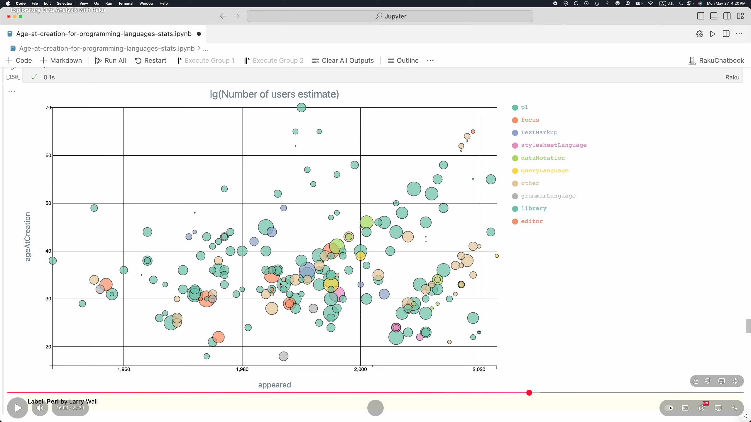
“Literate Programming (LP)” tooling is very important for doing Data Science (DS). At this point Raku has four LP solutions (three of them are “notebook solutions”):
The Jupyter Raku-kernel packages “Jupyter::Kernel” and “Jupyter::Chatbook” provide cells for rendering the output of LaTeX, HTML, Markdown, or Mermaid-JS code or specifications; see [AAv2].
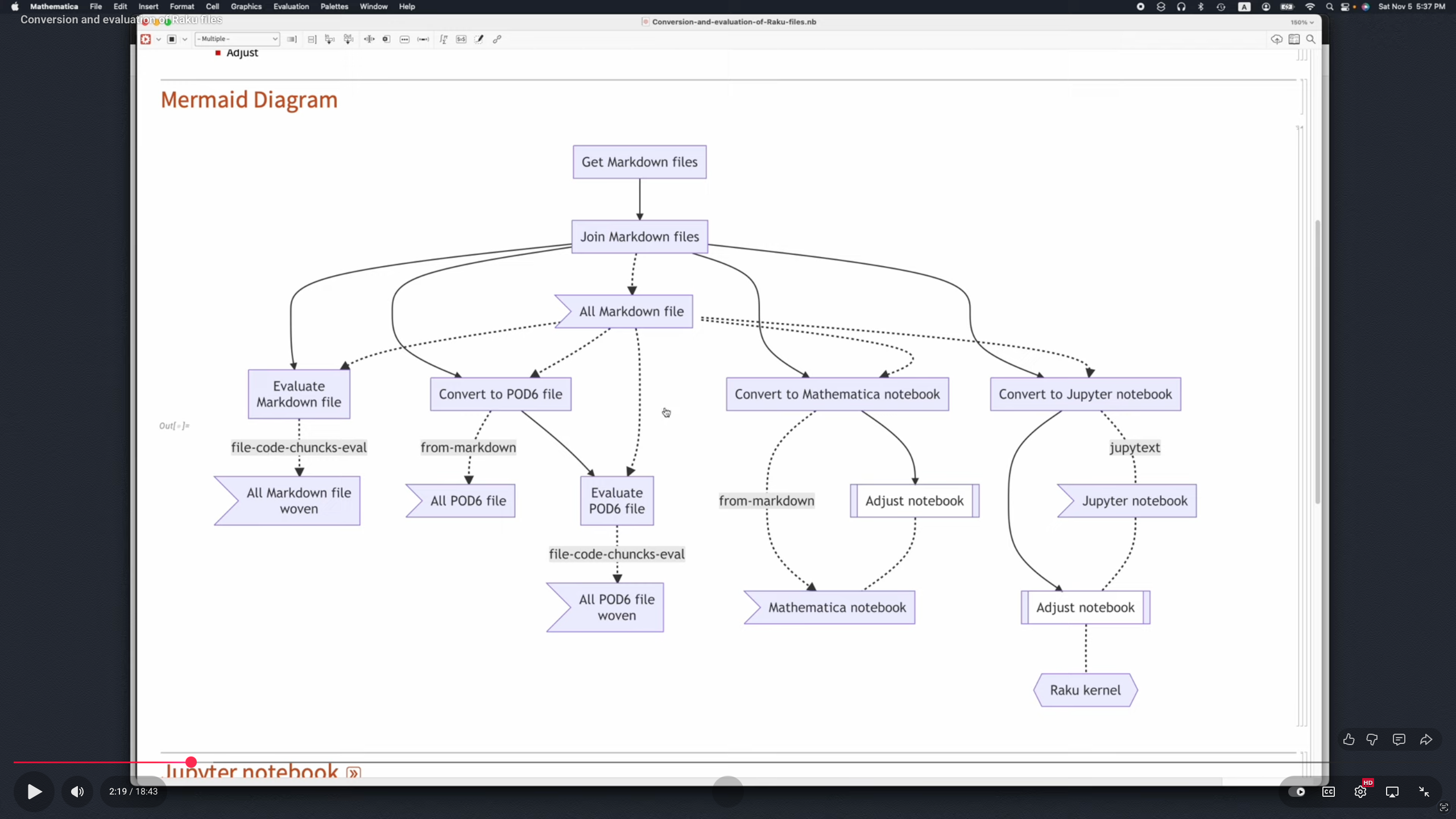
The package “Text::CodeProcessing” can be used to “weave” (or “execute”) computational documents that are Markdown-, Org-mode-, or Pod6 files; see [AAv2].
“RakuMode” is a Wolfram Language (WL) paclet for using Raku in WL notebooks. (See the next section for the “opposite way” — using WL in Raku sessions.)
Remark: WL is also known as “Mathematica”.
The package “Markdown::Grammar” can be used in notebook conversion workflows; see [AA1, AAv1].
Remark: This document itself is a “computational document” — it has executable Raku and Shell code cells. The published version of this document was obtained by “executing it” with the command:
A nice complement to the Raku’s DS and LLM functionalities is the ability to easily connect to other computational systems like Python, R, or Wolfram Language (WL).
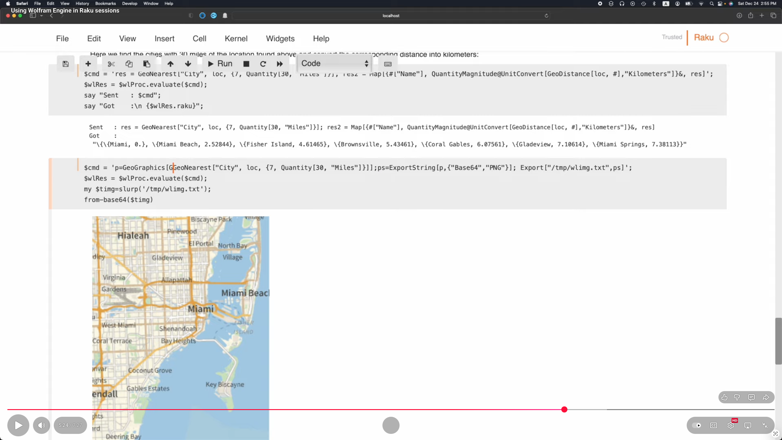
The package “Proc::ZMQed” allows the connection to Python, R, and WL via ZeroMQ; see [AAv3].
The package “WWW::WolframAlpha” can be used to get query answers from WolframAlpha (W|A). Raku chatbooks have also magic cells for accessing W|A; see [AA3].
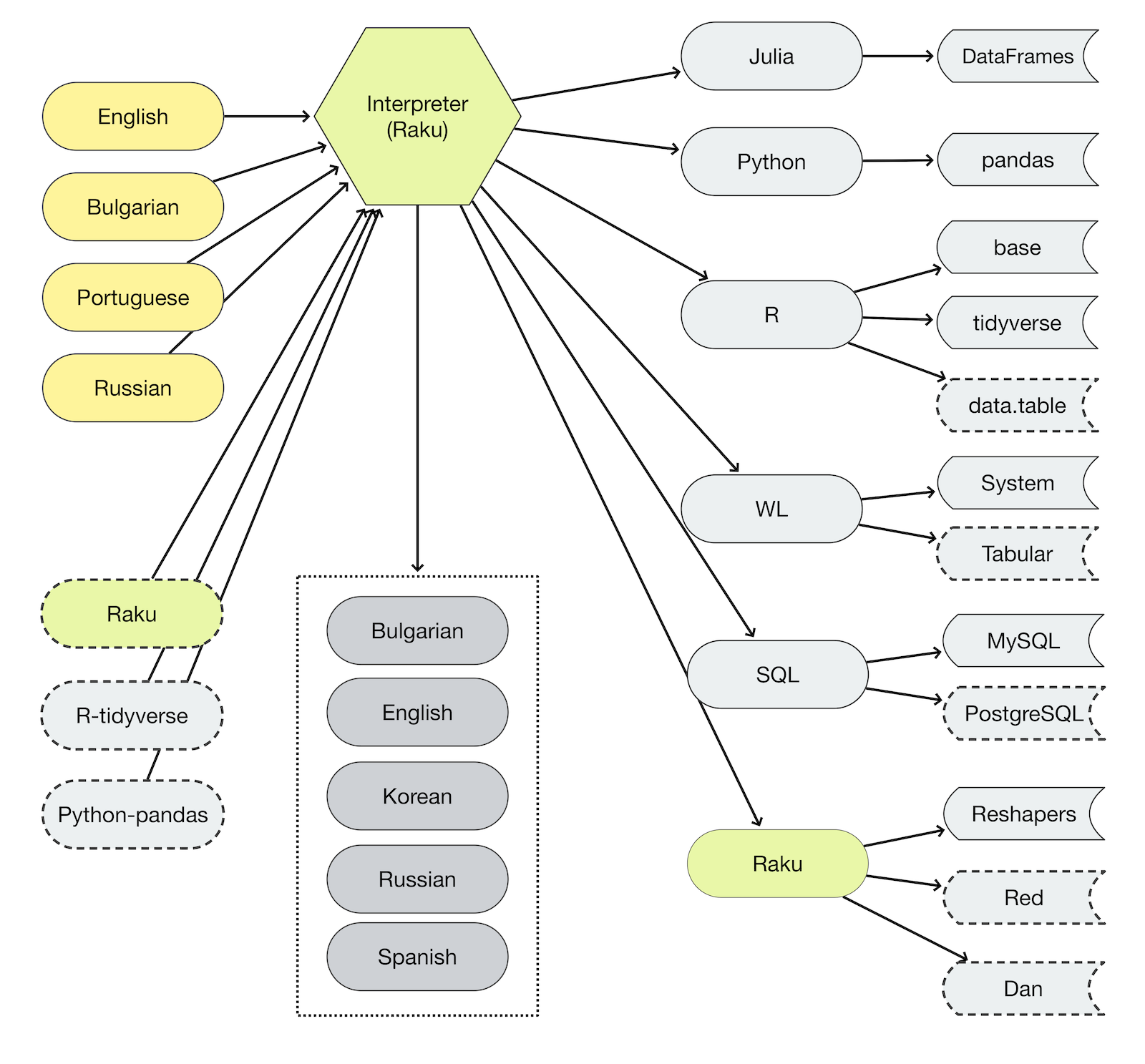
Cross language workflows
The packages listed in this document, along with the related articles and videos, support and demonstrate computational workflows that work across different programming languages.
Data wrangling workflows code generation is for Julia, Python, R, Raku, SQL, and Wolfram Language (WL).
Raku’s data wrangling functionalities adhere the DSLs and workflows of the popular Python “pandas” and R “tidyverse”.
More generally, ML workflows code generators as a rule target R, Python, and WL.
At this point, only recommender systems Raku-code is generated.
The Raku DSL for interacting with LLMs is also implemented in Python and WL; see [AAv8].
To be clear, WL’s design of LLM functions was copied (or transferred) to Raku.
Dancer, Dasher and the other reindeer work overtime on Christmas Eve delivering billions of gifts.
Each year the DevOps elves try and make things flow a bit smoother. The team use dosh (Do-Shell) – a Raku-powered command-line utility for turning natural language into platform-friendly shell commands.
Instead of remembering all those pesky command-line utilities and arguments, the DevOps team use dosh like this:
dosh asks your LLM of choice what to run — and returns a single, shell command with an explanation and warning if needed. It won’t execute the command without a human/elf confirming first.
Behind the scenes, dosh delegates its magic to the super-simple LLM::DWIM module and your $LLM of choice. dosh inserts the current operating system and architecture into the prompt for context. Use dosh prompt to see the current version of the prompt (v9):
You are a senior ubuntu shell engineer on linux 6.14.0-36-generic (x86_64).

Translate a natural-language request into ONE safe shell command for execution on the linux operating system.

RESPONSE FORMAT (STRICT):
Return MINIFIED JSON on a single line, with EXACT keys:
{"shell_command":"...","explanation":"...","warning":""}

RULES:
- shell_command: a single-line shell command that fully addresses the request.
- Prefer read-only substitutes (e.g., 'du -sh * | sort -h | tail -n 20') when user intent is unclear.
- NEVER include sudo unless essential; avoid destructive flags by default.
- NEVER access external services or APIs; use only local system commands instead.
- NEVER suggest a command that contains an http:// or https:// URL.
- explanation: a brief, friendly description of what the command does.
- warning: "" if read-only; otherwise 1 short sentence describing the risk.
- Output ONLY the minified JSON. No prose. No code fences. No backticks.

Examples:
{"shell_command":"ls -la","explanation":"Lists files with details in the current directory.","warning":""}
{"shell_command":"find . -type f -size +100M -print0 | xargs -0 ls -lh","explanation":"Shows paths and sizes of files larger than 100 MB.","warning":""}
{"shell_command":"find . -type f -name '*.bak' -delete","explanation":"Deletes all .bak files under the current directory.","warning":"This permanently removes files."}

The shell_command should solve the following command_request:

$your-request-goes-here
One of the junior Elves, who likes science fiction, was glad that a human/elf is always in the loop. Her testing showed:
How time flies. Yet another year has flown by. 2024 was a year of changes, continuations and preparations. Let’s start with the changes:
Edument
Edument Central Europe, the branch of Edument that is based in Prague (and led by Jonathan Worthington), decided to stop (commercial) development of its Raku related products: Comma (the IDE for the Raku Programming Language) and Cro (a set of libraries for building reactive distributed systems).
With the discrepancy between revenue and development cost to continue being so large, and the prevailing economic environment forcing us to focus on business activities that at least pay for themselves, we’ve made the sad decision to discontinue development of the Comma IDE.
Fortunately, Jonathan Worthington was not only able to release the final commercial version as a free download, but was also able to release all of the sources of Comma. This would allow other people to continue Comma development.
When Edument employees were by far the dominant Cro contributors, it made sense for us to carry the overall project leadership. However, the current situation is that members of the Raku community contribute more. We don’t see this balance changing in the near future.
With that in mind, we entered into discussions with the Raku Steering Council, in order that we can smoothly transfer control of Cro and its related projects to the Raku community. In the coming weeks, we will transfer the GitHub organization and release permissions to steering council representatives, and will work with the Raku community infrastructure team with regards to the project website.
As the source code of Cro had always been open source, this was more a question of handing over responsibilities. Fortunately the Raku Community reacted: Patrick Böker has taken care of making Cro a true open source project related to Raku, and the associated web site https://cro.raku.org is now being hosted on the Raku infrastructure. With many kudos to the Raku Infra Team!
A huge thanks
Sadly, Jonathan Worthington also indicated that they would only remain minimally involved in the further development of MoarVM, NQP and Rakudo in the foreseeable future. As such, (almost) all of their modules were moved to the Raku Community Modules Adoption Center, where they were updated and re-released.
It’s hard to overstate the importance of Jonathan Worthington‘s work in the development and implementation of the Raku Programming Language. So on behalf of the current, past and future Raku Community members: Thank You!
Issues cleanup
At the beginning of October, Elizabeth Mattijsen decided to take on the large number of open Rakudo issues at that time: 1300+. This resulted in the closing of more than 500 issues: some just needed closing, some needed tests, and some could be fixed pretty easily.
They reported on that work in the Raku Fall Issue Cleanup blog post. Of the about 800 open issues remaining, almost 300 were marked as “fixed in RakuAST”, and about 100 were marked as “Will be addressed in RakuAST”. Which still leaves about 400 open because of other reasons, so there’s still plenty of work to be done here.
More cleanup: p6c
The original Raku ecosystem (“p6c”) is in the process of being completely removed. Since March 2023, the ecosystem was no longer being refreshed by zef. But it was still being refreshed by the Raku Ecosystem Archiver. But this stopped in August 2024, meaning that any updates of modules in that ecosystem would go unnoticed from then on.
At that time, every author who still had at least one module in the “p6c” ecosystem was given notice by creating an issue in the repository of the first of their modules in the META.list. Luckily many authors responded, either by indicating that they would migrate their module(s) to the “zef” ecosystem, or that they were no longer interested in maintaining.
Since then, most of the modules of the authors that responded, have been migrated. And work has started on the modules of the authors that did not respond. With the following results: at the beginning of 2024, there were still 658 modules in the “p6c” ecosystem (now 427, 35% less), by 230 different authors (now 138, 40% less).
Ecosystem statistics
In 2024, 558 Raku modules have been updated (or first released): up from 332 in 2023 (an increase of 68%). There are now 2304 different modules installable by zef by just mentioning their name. And there are now 12181 different versions of Raku modules available from the Raku Ecosystem Archive, up from 10754 in 2023, which means almost 4 module updates / day in 2024.
Rakudo
Rakudo saw about 2000 commits (MoarVM, NQP, Rakudo, doc) this year, which is about the same as in 2023. About one third of these commits were in the development of RakuAST (down from 75% in 2023).
Under the hood, behind the scenes
A lot of work was done under the hood of the various subsystems of Rakudo. So was the dispatcher logic simplified by introducing several nqp:: shortcuts, which made the dispatcher code a lot more readable and maintainable.
The Meta-classes of NQP and Raku also received a bit of a makeover, as most of them hadn’t been touched since the 2015 release: this resulted in better documentation, and some minor performance improvements. Support for TWEAK methods and a rudimentary dd functionality were also added to NQP.
The JVM backend also got some TLC in 2024: one under the hood change (by Daniel Green) made execution of Raku code on the JVM backend twice as fast!
Timo Paulssen made the interface with low-level debuggers such as gdb and lldb a lot less cumbersome on MoarVM, which makes adding / fixing MoarVM features a lot easier!
On the MoarVM backend the expression JIT (active on Intel hardware) was disabled by default: it was found to be too unreliable and did not provide any execution speed gains. This change made Rakudo on Intel hardware up to 5% faster overall.
Also on the MoarVM backend, Daniel Green completed the work on optimizing short strings started by Timo Paulssen and Bart Wiegmans, resulting in about a 2% speed improvement of the compilation of Raku code.
Work on the Remote Debugger (which so far had only been really used as part of Comma) has resumed, now with a much better command line interface. And can now be checked in the language itself with the new VM.remote-debugging method.
Some race conditions were fixed: a particularly nasty one on the lazy deserialization of bytecode that was very hard to reproduce, as well as some infiniloops.
A lot of work was done on making the Continuous Integration testing produce fewer (and recently hardly any) false positives anymore. Which makes life for core developers a lot easier!
New traits
Two new Routine traits were added to the Raku Programming Language in 2024.
is item
The is item trait can be used on @ and % sigilled parameters to indicate that a Positional (in the @ case) or an Associative (in the % case) is only acceptable in dispatch if it is presented as an item. It only serves as a tie-breaker, so there should always also be a dispatch candidate that would accept the argument when it is not itemized. Perhaps an example makes this more clear:
multi sub foo(@a)         { say "array" }
multi sub foo(@a is item) { say "item"  }
foo  [1,2,3];  # array
foo $[1,2,3];  # item
is revision-gated(“v6.x”)
The is revision-gated trait fulfils a significant part of the promise of the Raku Programming Language to be a 100-year programming language. It allows a developer to add / keep behaviour of a dispatch to a subroutine or method depending on the language level from which it is being called.
As with is item, this is implemented as a tie-breaker to be checked only if there are multiple candidates in dispatch that match a given set of arguments.
This will allow core and module developers to provide forward compatibility, as well as backward compatibility in their code (as long as the core supports a given language level, of course).
In its current implementation, the trait must be specified on the proto to allow it to work (this may change in the future), and it should specify the lowest language level it should support. An example of a module “FOO” that exports a “foo” subroutine:
unit module FOO;
proto sub foo(|) is revision-gated("v6.c") is export {*}
multi sub foo() is revision-gated("6.c") {
    say "6.c";
}
multi sub foo() is revision-gated("6.d") {
    say "6.d"
}
Then we have a program that uses the “FOO” module and calls the “foo” subroutine. This shows “6.d” because the current default language level is “6.d”.
use FOO;

foo();  # 6.d
However, if this program would like to use language level 6.c semantics, it can indicate so by adding a use v6.c at the start of the program. And get a different result in an otherwise identical program:
use v6.c;
use FOO;

foo();  # 6.c
John Haltiwanger has written an extensive blog post about the background, implementation and usage of the is revision-gated trait on Day 16, if you’d like to know more about it.
Language changes (6.d)
These are some of the more notable changes in language level 6.d: all of them add functionality, so are completely backward compatible.
Flattening
The .flat method optionally takes a :hammer named argument, which will deeply flatten any data structure given:
my @a = 1, [2, [3,4]];
say @a.flat;           # (1 [2 [3 4]])
say @a.flat(:hammer);  # (1 2 3 4)
One can now also use HyperWhatever (aka **) in a postcircumfix [ ] for the same semantics:
my @a = 1, [2, [3,4]];
say @a[*];   # (1 [2 [3 4]])
say @a[**];  # (1 2 3 4)
Min/max/minmax options
The .min / .max / .minmax methods now also accept the :by named argument to make it consistent with the sub versions, which should prevent unexpected breakage when refactoring code from a sub form to a method form (as the :by would previously be silently ignored in the method form).
say min <5 45 345>, :by(*.Str);  # 345
say <5 45 345>.min(*.Str);       # 345
say <5 45 345>.min(:by(*.Str));  # 345  ADDED
.are(Type)
The .are method now also accepts a type argument. If called in such a manner, it will return True if all members of the invocant matched the given type, and False if not. Apart from allowing better readable code, it also allows shortcutting if any of the members of the invocant did not match the given type. An example:
unless @args.are(Pair) {
    die "All arguments should be Pairs";
}
Language changes (6.e.PREVIEW)
The most notable additions to the future language level of the Raku Programming Language:
.nomark
The .nomark method on Cool objects returns a string with the base characters of any composed characters, effectively removing any accents and such:
use v6.e.PREVIEW;
say "élève".nomark;  # eleve
:smartcase
The .contains / .starts-with / .ends-with / .index / .rindex / .substr-eq methods now all accept a :smartcase named argument: a conditional :ignorecase. If specified with a True value, it will look at the needle to see if it is all lowercase. If it is, then :ignorecase semantics will be assumed. If there are any uppercase characters in the needle, then normal semantics will be assumed:
use v6.e.PREVIEW;
say "Frobnicate".contains("frob");              # False
say "Frobnicate".contains("frob", :smartcase);  # True
say "Frobnicate".contains("FROB", :smartcase);  # False
IO::Path.stem
The .stem method on IO::Path objects returns the .basename of the object without any extensions, or with the given number of extensions removed:
use v6.e.PREVIEW;
say "foo/bar/baz.tar.gz".IO.basename;  # baz.tar.gz
say "foo/bar/baz.tar.gz".IO.stem;      # baz
say "foo/bar/baz.tar.gz".IO.stem(1);   # baz.tar
RakuAST
About one third of this year’s work was done on the RakuAST (Raku Abstract Syntax Tree) project. It basically consists of 3 sub-projects, that are heavily intertwined:
Development of RakuAST classes that can be used to represent all aspects of Raku code in an object-oriented fashion.
Development of a grammar and an actions class to parse Raku source code and turn that into a tree of instantiated RakuAST objects.
Development of new features / bug fixing in the Raku Programming Language and everything else that has become a lot easier with RakuAST.
RakuAST classes
There is little more to say about the development of RakuAST classes other than that there were 440 of them at the start of the year, and 454 of them at the end of the year. As the development of these classes is still very much in flux, they are not documented yet (other than in the test-files in the /t/12rakuast directory).
On the other hand, the RakuAST::Doc classes are documented because they have a more or less stable API to allow for the development of RakuDoc Version 2.
Raku Grammar / Actions
The work on the Raku Grammar and Actions has been mostly about implementing already existing features. This is measured by the number of Rakudo (make test) and roast (make spectest) test-files that completely pass with the new Raku Grammar and Actions. And these are the changes:
make test: 110/151 (72.8%) → 140/156 (89.7%)
make spectest: 980/1356 (72.3%) → 1155 / 1359 (85%)
A lot of work was done by Stefan Seifert, picking up the compile-time handling refactor that Jonathan Worthington had started in 2023, but was unable to bring to fruition. TPRF continued the funding for this work.
By the way, DuckDuckGo donated US$ 25000 to the foundation to allow this type of development funding to go on! Hint, hint!
Like last year, there are still quite a few features left to implement. Although it must be said that many tests are hinging on the implementation of a single feature, and often cause an “avalanche” of additional test-files passing when it gets implemented.
If you’d like to try out the new Raku Grammar and Actions, you should set the RAKUDO_RAKUAST environment variable to 1. The .legacy method on the Raku class will tell you whether the legacy (older) grammar is being used or not:
A cousin language was created: Draig, allowing you to write Raku code in Welsh!
Syntax Highlighting
The RakuAST::Deparse::Highlight module allows customizable Raku syntax highlighting of Raku code that is syntactically correct. It is definitely not usable for real-time syntax highlighting as it a. requires valid Raku code, and b. it may execute Raku code in BEGIN blocks, constant specifications and use statements.
A more lenient alternative is the Rainbow module by Patrick Böker.
RakuDoc
The final version of the RakuDoc v2.0 specification can now be completely rendered thanks to the tireless work of Richard Hainsworth and extensive feedback and proofreading by Damian Conway, as shown in Day 1 and Day 14.
Conference / Core Summit
Sadly it has turned out to be impossible to organize a Raku Conference (neither in-person or online), nor was it possible to organize a Raku Core Summit. We’re hoping for a better situation in 2025!
Amongst all of its features, what do we consider to be the essence of Raku? In this advent post we will explore what makes Raku an exciting programming language and see if we can describe its essence.
Who will design the languages of the future? One of the most exciting trends in the last ten years has been the rise of open-source languages like Perl, Python, and Ruby. Language design is being taken over by hackers. The results so far are messy, but encouraging. There are some stunningly novel ideas in Perl, for example. Many are stunningly bad, but that’s always true of ambitious efforts. At its current rate of mutation, God knows what Perl might evolve into in a hundred years.
Larry Wall took Paul Graham’s essay and ran with it:
“It has to do with whether it can be extensible, whether it can evolve over time gracefully.”
Larry referred to the expressiveness of human languages as his inspiration for Raku:
Languages evolve over time. (“It’s okay to have dialects…”)
No arbitrary limits. (“And they naturally cover multiple paradigms”)
External influences on style.
Fractal dimensionality.
Easy things should be easy, hard things should be possible.
“And, you know, if you get really good at it, you can even speak CompSci.”
Raku is a high-level, general-purpose, gradually typed language. Raku is multi-paradigmatic. It supports Procedural, Object Oriented, and Functional programming.
Object-oriented programming including generics, roles and multiple dispatch
Functional programming primitives, lazy and eager list evaluation, junctions, autothreading and hyperoperators (vector operators)
Parallelism, concurrency, and asynchrony including multi-core support
Definable grammars for pattern matching and generalized string processing
Optional and gradual typing
In Search of the Essence
As we can see, Raku has many rich features. Maybe the essence of Raku lies somewhere among them.
Deep Unicode
It’s the 21st Century and programming languages are finally waking up to the fact that we live in a multi-lingual world. Raku is a Unicode centric language in a way that no other language manages.
Rich Concurrency
Again programming languages are only beginning to catch up with the reality that every computer has multiple cores. Sometimes very many cores. Raku excels, alongside other modern languages, at delivering the tools required for effective concurrent and asynchronous programs.
Many languages in the same execution unit. No need to be an async/ IPC boundary away.
Representational polymorphism
The breadth of the Raku language is indeed impressive. But I don’t think it’s instructive, or even possible to try and distill an essence from such a diverse list of capabilities.
What then, is the Essence of Raku?
Perl and Raku both adhere to the famous motto:
TMTOWTDI (Pronounced Tim Toady): There is more than one way to do it.
This is indeed demonstrably true as shown by Damian Conway whenever he blogs about or talks about Raku. Indeed in Why I love Raku he sums up with this endorsement:
More than any other language I know, Raku lets you write code in precisely the way that suits you best, at whatever happens to be your (team’s) current level of coding sophistication, and in whichever style you will later find most readable …and therefore easiest to maintain.
How do you identify the essence of a deliberately broad multi-paradigm language? Perhaps the essence is not so much about some aspect of the core language. Perhaps it is much more about the freedom it gives you to choose, instead of the language choosing for you.
Like Raku, the community is not opinionated. If you choose a particular approach, the community is there to help you. If you want to learn what’s possible, the community will offer up multiple approaches, as shown by many Stack Overflow answers.
Which leaves me with this thought:
The essence of Raku is the freedom to choose for yourself. And the freedom to choose differently tomorrow.
Elf Nebecaneezer (‘Neb’) was welcoming some young new workers to his domain and doing what old folks like to do: pontificate. (His grandchildren politely, but behind his back, call it “bloviating.”)
“In the old days, we used hand-set lead type, then gradually used ever-more-modern methods; now we prepare the content in PDF and send a copy to another company to print the content on real newsprint. It still takes a lot of paper, but much less ink and labor (as well as being safer1).”
“Most young people are very familiar with HTML and online documents, but, unless your browser and printer are very fancy, it’s not easy to create a paper copy of the thing you need to file so that it’s very usable. One other advantage of hard-copy products is that they can be used without the internet or electricity. Remember, the US had a hugely-bad day recently when a major internet service provider had a problem!” [He continued to speak…]
Inspiration and perspiration
Now let’s get down to ‘brass tacks.’ You all are supposed to be competent Raku users, so I will show you some interesting things you can do with PDF modules. But first, a little background on PDF (Adobe’s Portable Document Format).
The PDF was developed by the Adobe company in 1991 to replace the PostScript (PS) format. In fact, The original PS code is at the heart of PDF. Until 2008, Adobe defined and continued to develop PDF. Beginning in 2008, the ISO defined it in its 32000 standard. That standard is about a thousand pages long and can be obtained online at https://www.pdfa-inc.org at no cost.
One other important piece of the mix is the CLI ghostscript interpreter which can be used, among other things, to compress PDF documents.
Before we continue, remember, we are a Debian shop, and any specific system software I mention is available in current versions.
Document creation
We are still improving Rakudoc (see the recent Raku Advent post by Richard Hainsworth), but it can be used now for general text to produce PDF output. However, for almost any specific printed product needed, we can create the PDF on either a one-time case or a specific design for reuse.
A good example of that is the module PDF::NameTags which can be modified to use different layouts, colors, fonts, images, and so forth. Its unique output feature is its reversibility–when printed two-sided, the person’s name shows regardless of whether the badge flips around or not. That module was used to create the name tags we are are wearing on our lanyards, and I created that module! I’ll be using parts of that module as an example as I continue.
Actually, I have a GitHub account under an alias, ‘tbrowder’, and I have published several useful modules to help my PDF work. I’ll mention some later.
Note I always publish my finished modules via ‘zef’, the standard Raku package manager. Then they are easily available for installation, and they automatically get listed on https://Raku.land and can easily be found. Why do I do that, especially since no one else may care? (As ‘@raiph’ or someone other Raku user once said, modules are usually created for the author’s use.) Because, if it helps someone else, as the Golden Rule says, it may be the right thing to do (as I believe Font::Utils does).
Fonts
Fonts used to be very expensive and hard to set type with, so the modern binary font is a huge improvement! Binary fonts come in different formats, and their history is fascinating.
This shop prefers OpenType fonts for two practical reasons: (1) they provide extensive Unicode glyph coverage for multi-language use (we operate world-wide as you well know) and (2) they provide kerning for more attractive type setting.
By using the HarffBuzz library, the final PDF will only contain the glyphs actually used by the text (the process is called ‘subsetting’). If a user is not running Debian 12 or later, then he or she can additionally ‘use’ module Compress::PDF which provides a subroutine which uses Ghostscript to remove unused glyphs. The module also provides a CLI program, pdf-compress, which does the same thing.
For Latin and most European languages we use the following font collections available as Debian packages:
Font
Debian package
GNU Free Fonts
fonts-freefont-otf
URW Base 35,
fonts-urw-base35
E B Garamond
fonts-egaramond, fonts-garamond-extra
Cantarell
fonts-cantarell
For other languages we rely on the vast glyph coverage of Google’s Noto fonts (in TrueType format). Debian has many of those fonts, but we find it easier to find the needed font at Google and download them onto our server as zip archives. After unzipping, we move the desired files to ‘/usr/local/share/fonts/noto’. We currently have these 10 Noto fonts available (plus 175 other variants):
Font
NotoSerif-Regular.ttf
NotoSerif-Bold.ttf
NotoSerif-Italic.ttf
NotoSerif-BoldItalic.ttf
NotoSans-Regular.ttf
NotoSans-Bold.ttf
NotoSans-Italic.ttf
NotoSans-BoldItalic.ttf
NotoSansMono-Regular.ttf
NotoSansMono-Bold.ttf
Note the file names above are in the family and style order as the Free Fonts in our own $HOME directory.
To get a feel for the span of glyphs in some of the fonts, the FreeSerif font has over 1,000 glyphs and can be used for many languages. We typically use that font, and the rest of that font family, for most of our work around Europe and the Americas. For the rest of the world, Google’s Noto fonts should cover all but a tiny fraction of the population.
One of the many strengths of Raku is its handling of Unicode as a core entity. You can read about Unicode at its website. Of particular interest are the code charts at https://www.unicode.org/charts. If you select any chart you will see that the code points are shown in hexadecimal. In Raku the code points are natively in decimal. Fortunately, Raku has a method to do that:
# convert decimal 178 to hexadecimal (base 16)
say 178.base(16); # OUTPUT: B2
# convert a hexadecimal 'A23' to decimal
say 'A23'.parse-base(16); # OUTPUT: 2595
Or we can look at Wikipedia where there are charts showing both hexidecimal and decimal code points (Unicode_chars).
Not released yet is my Raku module PDF::FontCollection which encapsulates useful font collections into a single reference list. The module has routines allowing the user to get a loaded font with a short code mnemonically associated with the font collection (a digit, and a one- or two-letter character for its style). It has an installed binary to show its fonts by number, code, and name. However, my most useful module, Font::Utils, has made this module effectively obsolete.
I now introduce my almost-released module Font::Utils which uses fonts already installed and collects them into a file called font-files.list which is then placed into the user’s $HOME/.Font-Utils directory.
Since our servers already have the desired OpenType fonts installed, using Font::Utils is actually more convenient since you can arrange the font list any way you want including: (1) creating your own mnemonic keys for easy reference, (2) deleting or adding data lines, and (3) reordering data lines.
Note that the actual OpenType font files are quite large, but a good design will ensure they are not loaded until specifically called for in the program. If they are already loaded, calling the routine will be is a no-op. The Font::Utils module has one such routine.
Other non-Latin languages are covered in many freely available font collections, including right-to-left and other orientations along with layouts for users who need that capability (the Noto fonts are a good example). As noted, those can be easily added to your Font::Utils collection.
Let’s take a look at the first couple of lines in the default installation of my $HOME/.Font-Utils/font-files.list:
We see the comments and the first line of data consisting of three fields. The first field is the unique code which you may change. The second field is the font file’s basename, and the last field is file font file’s path. You may delete or reorder or add new font entries as you wish.
Now let’s say you want to publish some text in Japanese. Oh, you say you don’t know Japanese? And you don’t have a keyboard to enter the characters? No problem!, There is a way to do that.
We first find from Wikipedia that some Unicode characters for the Japanese language are in the Hiragan collection, which covers hexadecimal code points 3041 through 3096 and 3099 through 309F. Then we create a space-separated string of the characters for each word. We’ll use an arbitrary list of them:
my $jword1 = "3059 306A 306B 306C 305D";
my $jword2 = "3059-305D"; # same as $jword1 but with a hyphen for a range
my $jword3 = "306B-306F";
Note that we can use a hyphen to indicate a contiguous range of code points. (We could also use decimal code points, but that’s a bit more awkward due to ease and larger number of characters required as well as the confusing use of the joining ‘-‘ with subtraction.)
Oops, what font shall we use? I couldn’t find a suitable font with the searches on Debian, so I went online to Google, searched for Hiragana, and found the font with description Noto Serif Japanese.
I selected it, downloaded it, and got file Noto_Serif_JP.zip. I created a directory named google-fonts and moved the zip file there where I then unpacked them to get directory Noto_Serif_JP with files:
The main font is a variable one, so I tried it to see the results.
Text
There are many ways to lay out text on a page. The most useful for general use is to create reusable text boxes.
Reusable text boxes
# define it
my PDF::Content::Text::Box $tb .= new(
   :$text, :$font, :$font-size, :$height,
   # style it
   :WordSpacing(5), # extra spacing for Eastern languages
);
#...clone it and modify it...
$tb.clone(:content-width(200));
Use the $page.text context to print a box:
my @bbox;
$page.text: {
    .text-position = $x, $y;
    # print the box and collect the resulting bounding box coordinates
    @bbox = .print: $tb;
Graphics and clipping
I won’t go into it very much, but you can do almost anything with PDF. The aforementioned PDF::NameTags module has many routines for drawing and clipping. Another of my modules on deck is PDF::GraphicsUtils which will encompass many similar routines as well as the published PDF::Document module.
Tricks and hints for module authors
Create a run alias
I was having trouble with the variable syntax needed testing scripts as well as test modules. Raku user and author @librasteve suggested creating an alias to do that. The result from my .bash_aliases file;
alias r='raku -I.'      # adhoc script Raku run command
alias rl='raku -I./lib' # adhoc script Raku run command
Use a load test
I was having problems with modules once and @ugexe suggested always using a load test for checking all modules will compile. Now I always create a test script similar to this:
# file: t/0-load-test.t
use Test;
my @modules = <
  Font::Utils
  Font::Utils::FaceFreeType
  Font::Utils::Misc
  Font::Utils::Subs
>;

plan +@modules;

for @modules {
    use-ok $_, "Module $_ can be used okay";
}
And run it like this: r t/0*t
$ r t/0*t
# OUTPUT:
1..4
ok 1 - Module Font::Utils can be used okay
ok 2 - Module Font::Utils::FaceFreeType can be used okay
ok 3 - Module Font::Utils::Misc can be used okay
ok 4 - Module Font::Utils::Subs can be used okay
‘=finish‘
Use =finish to debug a LONG rakumod file. I use it when I’m in the process of adding a new sub or modifying one and commit some error that causes a panic failure without a clear message. I add the =finish after the first routine and see if it compiles. If it does I move the =finish line to follow the next sub, and so on.
When I do get a failure, I have a better idea of where the bad code is. Note I do sometimes have to reorder routines becaause of inter-module dependencies. It’s also a good time to move completely independent routines to a lower-level module as described next.
Encapsulate small, independent routines
Sometimes, as in Font::Utils, I create a single, long file with routines that are dependent on other routines so that it is difficult to tell what is dependent upon what. Then I start creating another, lower-level module that has routines that are non-dependent on higher level modules. You can see that structure in the load test output shown above.
Use the BEGIN phaser
Module authors often need access to the user’s $HOME directory, so use of the BEGIN phaser as a block can make it easier to access it from the Build module, as well as the base modules. Here is that code from the Font::Utils module:
unit module Font::Utils;

use PDF::Font::Loader :load-font;
our %loaded-fonts is export;
our $HOME is export = 0;
our $user-font-list is export;
our %user-fonts     is export;
BEGIN {
    if %*ENV<HOME>:exists {
        $HOME = %*ENV<HOME>;
    }
    else {
        die "FATAL: The environment variable HOME is not defined";
    }
    if not $HOME.IO.d {
        die qq:to/HERE/;
        FATAL: \$HOME directory '$HOME' is not usable.
        HERE
    }
    my $fdir = "$HOME/.Font-Utils";
    mkdir $fdir;
    $user-font-list = "$fdir/font-files.list";
}
INIT {
    if not $user-font-list.IO.r {
        create-user-font-list-file;
    }
    create-user-fonts-hash $user-font-list;
    create-ignored-dec-codepoints-list;
}
That BEGIN block creates globally accessible variables and enables easy access for any build script to either create a new user fonts list or check an existing one. The INIT block then uses a routine to create the handy %user-fonts hash after the Raku compilation stage enables it.
As @lizmat and others on IRC #raku always warn about global variables: danger lurks from possible threaded use. But our ‘use cases’ should not trigger such a problem. However, other routines may, and we have used a fancy module to help the problem: OO::Monitors by @jnthn. See it used to good effect in the class (monitor) Font::Utils::FaceFreeType.
Experiment: Embedded links
Currently the PDF standard doesn’t deal with active links, but my Raku friend David Warring gave me a solution in an email. I think I’ve tried it, and I think it works, but YMMV.
David said “Hi Tom, Adding a link can be done. It’s a bit lower level than I’d like and you need to know what to look for. Also needs PDF::API6, rather than PDF::Lite. I’m looking at the pdfmark documentation. It’s a postscript operator and part of the Adobe SDK. It’s not understood directly by the PDF standard, but it’s just a set of data-structures, so a module could be written for it. I’ll keep looking.”
His code:
# Example:
use PDF::API6;
use PDF::Content::Color :&color, :ColorName;
use PDF::Annot::Link;
use PDF::Page;

my PDF::API6 $pdf .= new;
my PDF::Page $page = $pdf.add-page;

$page.graphics: {
    .FillColor = color Blue;
    .text: {
        .text-position = 377, 515;
        my @Border = 0,0,0; # disable border display
        my $uri = 'https://raku.org';
        my PDF::Action::URI $action = $pdf.action: :$uri;
        my PDF::Annot::Link $link = $pdf.annotation(
            :$page,
            :$action,      # action to follow the link
            :text("Raku homepage"), # display text (optional)
            :@Border,
         );
    }
}
$pdf.save-as: "link.pdf";
Because of the artistic nature of our work, we often need to create our own modules for new products. In that event, we use module App::Mi6 and its binary mi6 to ease the labor of managing recurring tasks with module development. By using a logical structure and a dist.ini configuration file, the user can create Markdown files for display on GitHub or GitLab, test his or her test files in directories t and xt, and publish the module on ‘Zef/Fez’ with one command each.
By using my module Mi6::Helper, the author can almost instantly create a new module ‘git’ source repository with its structure ready to use app mi6 with much boiler plate already complete.
I’m also working on a dlint program to detect structural problems in the module’s git repository. It is a linter to check the module repo for the following:
Ensure file paths listed in the META6.json file match those in the module’s /resources directory.
Ensure all use X statements have matching depends entries in the META6.json file.
Ensure all internal sub module names are correct.
The linter will not correct these problems, but if there is interest, that may be added in a future release.
Party time: finale
Neb concluded his presentation:
“Bottom line: Raku’s many PDF modules provide fairly easy routines to define any pre-press content needed. Those modules continue to be developed in order to improve ease of use and efficiency. Graphic arts have always been fun to me, but now they are even ‘funner!'”.
Santa’s Epilogue
As I always end these jottings, in the words of Charles Dickens’ Tiny Tim, “may God bless Us, Every one!” A Christmas Carol, a short story by Charles Dickens (1812-1870), a well-known and popular Victorian author whose many works include The Pickwick Papers, Oliver Twist, David Copperfield, Bleak House, Great Expectations, and A Tale of Two Cities2.
Footnotes
Old print shops: When I was in the seventh grade in my mother’s home town of McIntyre, Georgia, where we lived while my Dad was in Japan, we had a field trip to the local print shop of the Wilkinson County News. There the printer had to set lead type by hand, install the heavy frame set of type for the full page on the small, rotary press. Then he hand fed fresh newsprint paper as the apparatus inked the type-frame and then pressed the paper against the inked type. Finally, he removed the inked sheet and replaced it with the next copy. One of the kids noted the sharp pin on the press plate to hold the paper and asked if that ever caused problems. The printer showed us his thumb with a big scar and said that was the mark of an old time press man and just an expected hazard of the trade. ↩︎
A Christmas Carol, a short story by Charles Dickens (1812-1870), a well-known and popular Victorian author whose many works include The Pickwick Papers, Oliver Twist, David Copperfield, Bleak House, Great Expectations, and A Tale of Two Cities. ↩︎