Day 22 – Wrapping a Christmas Present

A few months back

In the smoke-filled (virtual) room of the council of the high (from the smoke) elves, the wizened textualist Geoff, said “All of my stuff is in boxes and containers.” Empty shelves behind him indicated he was moving house.

“When you have a complex module,” Geoff continued, “and its difficult to describe how to install it, do all the steps in a container, and show the Dockerfile.”

“Aha!” said the newest member, who drew his vorpal sword, and went forth to slay the Jabberwock, aka putting RakuAST::RakuDoc::Render into a container.

“Beware the Jabberwock, my son!
The jaws that bite, the claws that catch!”

After days of wandering the murky jungle of Docker/Alpine/Github/Raku documentation, the baffled elf wondered if he was in another fantasy:

“So many rabbit holes to fall down.”

Rabbit Hole, the First – alpinists beware

Best practice for a container is to chose an appropriate base image. Well obviously, there’s the latest Raku version by the friendly, hard-working gnomes at Rakuland. So, here’s the first attempt at a Dockerfile:

FROM docker.io/rakuland/raku
# Copy in Raku source code and build
RUN mkdir -p /opt/rakuast-rakudoc-render
COPY . /opt/rakuast-rakudoc-render
WORKDIR /opt/rakuast-rakudoc-render
RUN zef install . -/precompile-install

It failed. After peering at the failure message, it seemed that at least one of the dependent modules used by the rakuast-rakudoc-render distribution needs a version of make.

That’s easily fixed, just add in build-essentials, the vorpal-sworded elf thought. Something like:

FROM docker.io/rakuland/raku

# Install make, gcc, etc.
RUN apt-get update -y && \
    apt-get install -y build-essential && \
    apt-get purge -y

# Copy in Raku source code and build
RUN mkdir -p /opt/rakuast-rakudoc-render
COPY . /opt/rakuast-rakudoc-render
WORKDIR /opt/rakuast-rakudoc-render
RUN zef install . -/precompile-install

Failure! No apt.

“How can there not be APT??” the Ubuntu-using elf thought in shock. Turns out that the rakuland/raku image is built on an Alpine base, and Alpine have their own package manager apk.

Unfortunately, build-essential is a debian package, but at the bottom of this rabbit hole lurks an apk equivalent package build-base, leading to:

FROM docker.io/rakuland/raku

# Install make, gcc, etc.
RUN apk add build-base

# Copy in Raku source code and build
RUN mkdir -p /opt/rakuast-rakudoc-render
COPY . /opt/rakuast-rakudoc-render
WORKDIR /opt/rakuast-rakudoc-render
RUN zef install . -/precompile-install

Lo! upon using the Podman desktop to build an image from the Dockerfile, the process came to a succesful end.

But now to make things easier, there needs to be a link to the utility RenderDocs, which takes all the RakuDoc sources from docs/ and renders them to $*CWD (unless over-ridden by --src or --to, respectively). It will also render to Markdownunless an alternative format is given.

FROM docker.io/rakuland/raku

# Install make, gcc, etc.
RUN apk add build-base

# Copy in Raku source code and build
RUN mkdir -p /opt/rakuast-rakudoc-render
COPY . /opt/rakuast-rakudoc-render
WORKDIR /opt/rakuast-rakudoc-render
RUN zef install . -/precompile-install

# symlink executable to location on PATH
RUN ln -s /opt/rakuast-rakudoc-render/bin/RenderDocs /usr/local/bin/RenderDocs

# Directory where users will mount their documents
RUN mkdir /doc

# Directory where rendered files go
RUN mkdir /to
WORKDIR /

AND!!! when a container was created using this Dockerfile and run with its own terminal, the utility RenderDocs was visible. Running

RenderDocs -h

produced the expected output (listing all the possible arguments).

Since the entire distribution is included in the container, running

RenderDocs --src=/opt/rakuast-rakudoc-render/docs README

will render README.rakudoc in --src to /to/README.md because the default output format is MarkDown.

“Fab!”, screamed the boomer-generation newbie elf. “It worked”.

“Now lets try HTML”, he thought.

RenderDocs --format=HTML --src=/opt/rakuast-rakudoc-render/docs README

Failure: no sass.

expletive deleted“, he sighed. “The Jabberwok is not dead!”

There are two renderers for creating HTML. One produces a single file with minimal CSS so that a normal browser can load it as a file locally and it can be rendered without any internet connection. This renderer is triggered using the option --single. Which the containerised RenderDocs handles without problem.

Rabbit Hole, the second – architecture problems

But the normal use case is for HTML to be online, using a CSS framework and JS libraries from CDN sources. Since the renderer is more generic, it needs to handle custom CSS in the form of SCSS. This functionality is provided by calling an external program sass, which is missing in the container.

An internet search yields the following snippet for a container.

# install a SASS compiler
ARG DART_SASS_VERSION=1.82.0
ARG DART_SASS_TAR=dart-sass-${DART_SASS_VERSION}-linux-x64.tar.gz
ARG DART_SASS_URL=https://github.com/sass/dart-sass/releases/download/${DART_SASS_VERSION}/${DART_SASS_TAR}
ADD ${DART_SASS_URL} /opt/
RUN cd /opt/ && tar -xzf ${DART_SASS_TAR} && rm ${DART_SASS_TAR}
RUN ln -s /opt/dart-sass/sass /usr/local/bin/sass

The container image builds nicely, but the RenderDocs command STILL chokes with an unavailable sass.

Except that diving into the container’s murky depths with an ls /opt/dart-sass/ shows that sass exists!

The newbie was stumped.

So rested he by the Tumtum tree
And stood awhile in thought.

Turns out that the Alpine distribution uses a different compiler, and the wonderful dart-sass fae provide a suitable binary so a simple change was enough to get sass working in the container.

- ARG DART_SASS_TAR=dart-sass-${DART_SASS_VERSION}-linux-x64.tar.gz
+ ARG DART_SASS_TAR=dart-sass-${DART_SASS_VERSION}-linux-x64-musl.tar.gz

simple does not mean found at once, but the container contains RenderDocs, which produces markdown and HTML rendered files.

One, two! One, two! And through and through
The vorpal blade went snicker-snack!
He left it dead, and with its head
He went galumphing back.

“I can publish this image so everyone can use it,” the FOSS fanatic elf proclaimed.

So the docker container image can be accessed using a FROM or PULL using the URL

docker.io/finanalyst/rakuast-rakudoc-render

Rabbit Hole, the third – Versions

“And hast thou slain the Jabberwock?
Come to my arms, my beamish boy!
O frabjous day! Callooh! Callay!”

“It would be great,” mused the triumphant elf, “if RakuDoc sources, say for a README could be automatically included as the github README.md of repo”.

“May be as an action?”

Github actions can use containers to process files in a repo. Essentially, in an action, the contents of a repo are copied to a github-workspace, then they can be processed in the webspace, and changes to the workspace have to be committed and pushed back to the repository.

With a container, the contents of the workspace need to be made available to the container. Despite some documentation that starting a container in a github action automatically maps the github-workspace to some container directory, the exact syntax is not clear.

In order to discover how to deal with the multitude of possibilities, a new version of RenderDocs got written, and a new image generated, and again, and again … Unsurprisingly, between one meal and another, the ever hungry elf forgot which version was being tested.

“I’ll just include a --version argument,” thought the elf. “I’ll can ask the Super Orcs!”.

And there behold was an SO answer to a similar question, and it was written by no lesser a high elf than the zefish package manager ugexe, not to be confused with the other Saint Nick, the package deliverer.

Mindlessly copying the spell fragment into his CLI script as:

multi sub MAIN( :version($v)! = False {
    say "Using version {$?DISTRIBUTION.meta<version>} of rakuast-rakudoc-render distribution."
    if $v;
}

the elf thought all done! “Callooh! Callay!”.

Except RenderDocs -v generated Any.

“SSSSSSSSh-,” the elf saw the ominous shadow of Father Christmas looming, “-ine a light on me”.

On the IRC channel, the strong willed Coke pointed out that a script does not have a compile time variable, such as, $?DISTRIBUTION. Only a module does.

The all-knowing elf wizard @lizmat pointed out that command line scripts should be as short as possible, with the code in a module that exports a &MAIN.

Imbibing this wisdom, our protagonist copied the entire script contents of bin/RenderDocs to lib/RenderDocs.rakumod, added a proto sub MAIN(|) is export { {*} }, then made a short command line script with just use RenderDocs.

Inside the container terminal:

# RenderDocs -v
Using version 0.20.0 of rakuast-rakudoc-render distribution.

With that last magical idiom, our intrepid elf was ported from one rabbit hole back to the one he had just fallen down.

Rabbit Hole, the fourth – Actions

“Beware the Jubjub bird, and shun
The frumious Bandersnatch!”

“I seem to be going backwards,” our re-ported elf sighed.

Once again, the github documentation was read. After much study and heartbreak, our hero discovered a sequence that worked:

  1. Place Lavendar and sandalwood essential oils in a fragrance disperser
  2. Prepare a cup of pour over single-origin coffee with a spoon of honey, and cream
  3. In a github repo create a directory docs containing a file README.rakudoc
  4. In the same github repo create the structure
    .github/
        workflows/
            CreateDocs.yml
  1. Write the following content to CreateDocs.yml
    name: RakuDoc to MD
    on:
      # Runs on pushes targeting the main branch
      push:
        branches: ["main"]
      # Allows you to run this workflow manually from the
      # Actions tab workflow_dispatch:
    jobs:
        container-job:
            runs-on: ubuntu-latest
            steps:
                - name: Checkout code
                  uses: actions/checkout@master
                  with:
                    persist-credentials: false
                    fetch-depth: 0
                - name: Render docs/sources
                  uses: addnab/docker-run-action@v3
                  with:
                    image: finanalyst/rakuast-rakudoc-render:latest
                    registry: docker.io
                    options: -v ${{github.workspace}}/docs:/docs -v ${{github.workspace}}:/to
                    run: RenderDocs

After examining the github actions logs, it seemed the rendered files were created, but the repository was not changed.

“Perhaps I should have used milk and not cream …” thought our fantasy elf.

There is in fact a missing step, committing and pushing from the github-workspace back to the repository. This can be done by adding the following to CreateDocs.yml:

- name: Commit and Push changes
  uses: Andro999b/push@v1.3
  with:
    github_token: ${{ secrets.GITHUB_TOKEN }}
    branch: 'main'

Even this did not work! Github refused absolutely to write changes to the repository.

The weary elf substituted Lemon grass for Lavender in step 1, and just to be certain changed the repo settings following the instructions from the Github grimore 

  1. select Settings in the repo’s main page
  2. select Actions then General
  3. from the dropdown for GITHUB_TOKEN, select the one for read and write access.
  4. Save settings

The content – at this stage of the tale – of CreateDocs.yml is

name: RakuDoc to MD
on:
  # Runs on pushes targeting the main branch
  push:
    branches: ["main"]
  # Allows you to run this workflow manually from the Actions tab
  workflow_dispatch:
jobs:
    container-job:
        runs-on: ubuntu-latest
        steps:
            - name: Checkout code
              uses: actions/checkout@master
              with:
                persist-credentials: false
                fetch-depth: 0
            - name: Render docs/sources
              uses: addnab/docker-run-action@v3
              with:
                image: finanalyst/rakuast-rakudoc-render:latest
                registry: docker.io
                options: -v ${{github.workspace}}/docs:/docs -v ${{github.workspace}}:/to
                run: RenderDocs
            - name: Commit and Push changes
              uses: Andro999b/push@v1.3
              with:
                github_token: ${{ secrets.GITHUB_TOKEN }}
                branch: 'main'

It worked. “The Christmas present is now available for anyone who wants it”, thought our elf.

’Twas brillig, and the slithy toves
Did gyre and gimble in the wabe:
All mimsy were the borogoves,
And the mome raths outgrabe.
(Jabberwocky, By Lewis Carroll)

Remember to git pull for the rendered sources to appear locally as well.

Rabbit Hole, the fifth – Diagrams

“Wouldn’t it be nice to wrap the present in a ribbon? Why not put diagrams in the Markdown file? “

Our elf was on a streak, and fell down another rabbit hole: github does not allow svg in a Markdown file it renders from the repo. “It is impossible,” sighed the tired elf.

Alice laughed. “There’s no use trying,” she said: “one can’t believe impossible things.”
“I daresay you haven’t had much practice,” said the Queen. “When I was your age, I always did it for half-an-hour a day. Why, sometimes I’ve believed as many as six impossible things before breakfast.”
(Through the Looking Glass, Lewis Carroll)

Diagrams can be created using the dot program of Graphviz, which is a package that Alpine provides. So, we can create a custom block for RakuAST::RakuDoc::Render that takes a description of a graph, sends it to dot, gets an svg file back and inserts into the output.

Except: github will not allow svg directly in a markdown file for security reasons.

But: it will allow an svg in a file that is an asset on the repo. So, now all that is needed is to save the svg in a file, reference the file in the text, and copy the asset to the same directory as the Markdown text.

Except: the time stamps on the RakuDoc source files and the output files seem to be the same because of the multiple copying from the repo to the actions workspace to the docker container. So: add a --force parameter to RenderDocs.

So in Raku impossible things are just difficult.

The final content of CreateDocs.yml is now

name: RakuDoc to MD
on:
  # Runs on pushes targeting the main branch
  push:
    branches: ["main"]
  # Allows you to run this workflow manually from the Actions tab
  workflow_dispatch:
jobs:
    container-job:
        runs-on: ubuntu-latest
        steps:
            - name: Checkout code
              uses: actions/checkout@master
              with:
                persist-credentials: false
                fetch-depth: 0
            - name: Render docs/sources
              uses: addnab/docker-run-action@v3
              with:
                image: finanalyst/rakuast-rakudoc-render:latest
                registry: docker.io
                options: -v ${{github.workspace}}/docs:/docs -v ${{github.workspace}}:/to
                run: RenderDocs --src=/docs --to=/to --force
            - name: Commit and Push changes
              uses: Andro999b/push@v1.3
              with:
                github_token: ${{ secrets.GITHUB_TOKEN }}
                branch: 'main'

Try adding a graph to a docs/README.rakudoc in a repo, for instance:


=begin Graphviz :headlevel(2) :caption<Simple example>
    digraph G {
        main -> parse -> execute;
        main -> init;
        main -> cleanup;
        execute -> make_string;
        execute -> printf
        init -> make_string;
        main -> printf;
        execute -> compare;
    }
=end Graphviz

Now you will have a README with an automatic Table of Contents, all the possibilities of RakuDoc v2, and an index at the end (if you indexed any items using X<> markup).

(Sigh: All presents leave wrapping paper! A small file called semicolon_delimited_script is also pushed by github’s Commit and Push to the repo.)

Day 21 – Dam Mega Christmas

Source file: Le Grand PortageDerivative work: Rehman, CC BY 2.0 https://creativecommons.org/licenses/by/2.0, via Wikimedia Commons

[Edited by author]

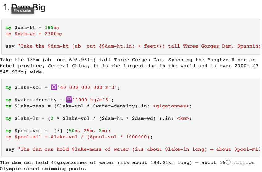
Scientists have also discovered that so-called megastructures built by humans can also affect the Earth’s rotation. Take the 185m (about 600 feet) tall Three Gorges Dam. Spanning the Yangtze River in Hubei province, Central China, it is the largest dam in the world and is over 2,300m (7,500 feet) in length.

Its vital statistics are dizzying. It was made using 28 million cubic metres of concrete and enough steel to build 63 copies of the Eiffel Tower. It took 40,000 people 17 years to construct, at a total cost of $37 billion (£28 billion). The dam can hold 40 billion cubic metres of water – about 16 million Olympic-sized swimming pools.

Dam, thought Rudolph (for he was prone to silent cursing). He was worried that this may confuse Santa’s SaNtav (ed – that’s a stretch!).

He decided to flex his Raku skills there and then and to check this nonsense once and for all. Luckily with his friends Anton and Ab5stract, he had the full power of the IntelliJ JetBrains Raku Plugin (the plugin formerly known as Comma) and Jupyter::Chatbook and could fire up a Jupyter Raku notebook in a jiffy.

IntelliJ Jetbrains Comma Raku Plugin

He loved it when his hooves hit the keyboard and he was able to get all that cool IDE shit:

  • Jupyter Raku kernel alongside Python
  • Raku Syntax highlighting in notebook cells
  • Latex and all manner of Jupyter cell magics
  • Out of this world LLM cell magic

But Rudi wanted even more power – he wanted to calculate some awesome numbers and needed a tool to keep him straight in his Physics.

Physics::Measure

Wait, right there in a notebook he could use the raku Physics::Measure module…

zef Physics::Measure did the trick.

And here’s how it went…

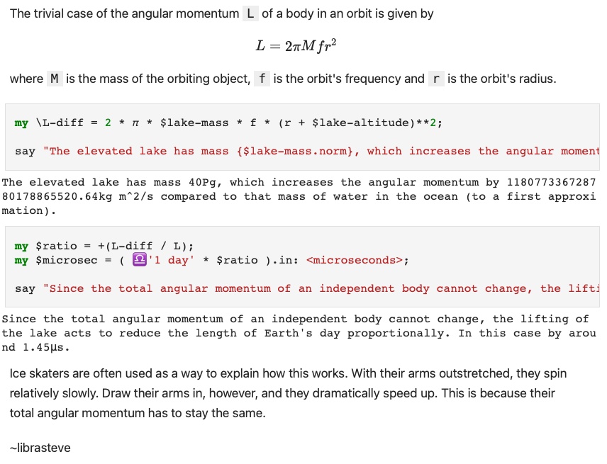
sorry about the images and the spill to the right margin for legibility here – please go here to copy and paste into your own notebook … meantime it may help to embiggen your browser view

Dam Close Call

Phew thought Rudolph – if I can just dial in the differential of 1.45µsec to the SaNtav (groan!). But, then he noticed that his hooves were too big to dial in the new numbers…

~librasteve

with inspiration from here.

PS. the full text, docker instances, installation instructions and example code is here if you want to emulate Rudolph – https://github.com/librasteve/raku-Physics-Measure-Jupyter

PPS. As a stretch goal, a mince pie to the first comment below that shows how to make a custom Physics::Measure unit called the mega-pool.

Day 20 – Re-introducing a Raku plugin for IntelliJ IDEA

Ever since its release back in the distant universe of 2018, I was a big fan and paying user of Comma IDE. Produced by the lovely folks over at Edument, Comma was both a full-fledged, standalone IDE as well as a plugin for IntelliJ IDEA-based IDEs.

In reality the standalone version and the plugin shared the same code. The standalone Comma IDE represented a mostly rare third-party derivation of the IntelliJ IDEA Community open source platform, whereas the plugin used the more common approach of simply extending the IntelliJ IDEA applications provided by JetBrains directly.

Unfortunately as times moved on, it had reportedly become more and more difficult for Edument to align the costs of keeping up with the continuously evolving IntelliJ platform with the income generated by the Comma offerings. You can read more about that in the official announcement of Comma’s development coming to an end.

A second life for Comma

While it was obviously sad news to hear about the discontinuation of Comma as a commercial product, the community was blessed by a source release of the plugin code. In combination with the forked version of the IntelliJ Community source (intellij-ide-fork), it was once again technically possible for the community to re-create Comma in both IDE and plugin form.

I kept that very possibility in the back of my mind as the days, weeks, and months ticked over after the discontinuation announcement in February. I have learned to tolerate Java as a result of my $day-job, but I was also willing to wait and see if some other willing soul would appear and revive Comma (in the words of management’s clueless response to revelations of efforts that required overtime, “work smarter, not harder”).

By August, however, I had the tuits to take the efforts up myself and so dove into trying to re-create the standalone Comma IDE.

The pace of change is certainly a thing

I quickly collided into a hard truth about the era of IntelliJ Community that Comma IDE was built against. The comma-223.4884 branch of intellij-ide-fork is 79,982 commits behind the code in the intellij-comunity repository. Those ~80k commits represent only about 24 months of activity. That’s a lot of change!

One of the most crucial changes that was being undertaken over those months, and actually over several years preceding them, was the transition from a build system called JPS to the Gradle IntelliJ Plugin. From what I understand, JPS requires a local checkout fo intellij-community (or a custom fork such as we find in intellij-ide-fork) — something that the Gradle IntelliJ Plugin does not.

Unfortunately, there is no current way to use Gradle IntelliJ Plugin to build a standalone IDE. (The documentation implies that this is an eventual goal, but I’ve heard that this page has been in place for years without update).

I spent two weeks trying and failing to make any sensible progress with JPS and a checkout of intellij-ide-fork rebased onto the latest intellij-community before finally setting aside the dream of a standalone Comma (for now…).

Catching up

After switching over to the Gradle Intellij Plugin, progress went from non-existent to quite fast-paced. Switching from targeting standalone to developing a plugin was clearly the right choice for the moment.

There was another course correction which completely transformed the velocity of change…

IntelliJ provides an option in the Code menu: Convert Java File to Kotlin File. They should put up a warning that any current tolerance levels for writing Java code will almost certainly decrease precipitously. I know mine did! There’s just zero reason — in this or any universe — to start a new codebase in Java when you can write Kotlin and integrate with Java libraries seamlessly.

At some point I’m going to try the same trick with the Java implementation of NQP.

A somewhat complete list of changes

  • All references of Perl 6 replaced with Raku.
  • 49 Annotations were rewritten as Inspections, along with 34 associated Fixes.
    • Inspections can be selectively enabled/disabled from the IntelliJ settings.
  • New Raku project setup that uses the latest Kotlin UI DSL instead of deprecated internals.
  • Complete rewrite of META6.json handling based on Kotlin serialization.
  • Introduced a service that checks if the project contains the core Rakudo source.
    • If so, it prompts the user whether they want to disable a handful of inspections that can get thrown off by core source code (such as attributes introduced in the bootstrap but used in the class source).
  • Major cleanup and revision of services in general.
  • Complete rewrite of fetching the ecosystem.
  • Complete rewrite of package management.
  • Migration of storing the Raku SDK to today’s recommended approach.
  • Added NQP syntax highlighting.
  • Added ‘🦋’ menu for quickly setting the Raku SDK version and launching REPLs.

A few of the things yet to be addressed

  • Comma had quite a comprehensive test suite. Reanimate it!
  • Validate that all Cro-specific functionality is working as expected.
  • Look into some highlighting related parser issues.
  • Fix dependency management for names that use :auth, :ver, etc.
  • Add a UI for installing modules.
  • Migrate as many Java files to Kotlin as possible (some that need static can’t be reasonably converted yet)
  • Publish to the Jetbrains Marketplace.
  • Migrate the repo to the github.com/Raku community namespace.
  • Include some additional themes, if possible.

What’s in a name?

We’ve been calling the revitalized plugin comma-plugin 2.0. However, in consultation with Jonathan Worthington and with current users, the plan is to rename the plugin to simply Raku before publishing to the Jetbrains Marketplace.

This aligns with the naming scheme of most other programming language plugins for IntelliJ. It does have the disadvantage of being harder to reference in communication. Therefore I somewhat expect to keep using Comma or perhaps The Plugin to refer to the efforts in IRC and elsewhere.

Concluding thoughts

IntelliJ IDEA is a fast-moving target and coding a plugin for it has enlightened me to some of the dynamics that probably contributed to the cancellation of Comma as a commercial product.

That said, the IntelliJ IDEA Platform is quite a pleasure to code against. It is generally well-documented and has clearly benefited from two decades of evolution. That always carries some baggage but for the most part I felt like I was working with a really well-designed ecosystem of IDE subsystems.

Kotlin is an incredible leap forward for working with legacy Java code and the JVM. I was feeling like my Java code was hitting a decent stride in terms of concision and expressiveness.

After my fateful decision to use IntelliJ’s automatic Java-to-Kotlin converter, that feeling has significantly evaporated. Writing Java is back to feeling hopelessly verbose, even in its sharpest forms. (Forget about JDK < 17! Instead, write Kotlin and target those ancient versions instead.)

So, approach Kotlin with caution if you’re going to be forced to write Java at work. It’s still worth it, in my opinion. I’ll have to write some posts about what I like about it some other time.

Interested in giving the Raku plugin for IntelliJ a try? Please check out the source or download the latest release.

Day 19 – Wrapping Scripts

This is a cross post of https://dev.to/patrickbkr/better-wrapper-scripts-158j

When creating an application in Raku one will at one point typically hit the issue that the application can only be started by calling raku and passing a few arguments. The usual solution is to write a small wrapper shell script on POSIX and a bat script on Windows. But getting these wrapper scripts really right is not trivial. Typical pitfalls are:

  • The script depends on the current working directory
  • It requires Bash and thus can’t work in e.g. BusyBox
  • It fails to process args that contain special chars (e.g. < or > (or many others) combined with bat files is fun)
  • It insta returns to the prompt and then ghost writes to the terminal on Windows

A few years ago I started working on a tool to help generating robust wrappers for this use case. I’ve finally pushed it over the finish line.

I’ve named it the Executable Runner Generator. The name could have been chosen better, but we’ll have to live with it now. It’s written in Raku, but the generated wrappers are independent of the language. Currently it can generate wrappers that work on Windows x86_64 and all sorts of POSIX systems.

In general the task of the wrapper is to put together a command line (and runtime environment like CWD and env vars) and execute the program. How exactly that happens is configured via a set of options. The wrapper has the ability to:

  • Construct paths relative to the wrappers file system location
  • Change path separators on Windows
  • Change the current working directory
  • Specify the command line arguments to pass to the program
  • Forward the arguments passed to the wrapper
  • Add and remove environment variables

How?

Glad you asked! To install run

zef install Devel::ExecRunnerGenerator

Then create a file my-app-runner-config.json with these contents:

program => "<abs>bin/raku",
cwd => "<abs>.",
args => [
    "<abs>share/perl6/site/bin/my-app.raku",
    "<cmd-args>"
],
archs => [
    "posix",
    "windows-x86_64.exe",
],
out-path => ".",
:overwrite

Now run

exec-runner-generator --config=my-app-runner-config.json

Which should leave you with a posix and windows-x86_64.exe file. Congratulations!

For all the non-Raku folks out there, there even is a small webservice that exposes the functionality: https://boekernet.de/erg

Happy adventing everyone!

P.S.
On Windows the generator relies on a native executable written in C to do its magic. There is no exec syscall on Windows. The program works around this by staying alive, letting the child process inherit its file descriptors and once the child finishes, returns with its exit code.

I’m pretty sure this “exec emulation” isn’t perfect. But as I’m not a Windows low level expert I don’t even know what I’m missing. Signals? Security contexts? I don’t know.
So: If you are knowledgeable of the lower Windows APIs, I’d love to get feedback on the implementation or maybe even a patch. You can reach me on many channels.

Day 18 – Happy™ Xmas

Christmas was fast approaching and Santa was starting to worry about all the presents being wrapped in time. Ensuring that he could quickly find the Elfmail address for all of the team was important to whip them into shape.

Luckily, Rudolph [for it was he] had been learning raku and cro for some years now and he was ready to help. This year he had read about the wonderful HTMX framework and thought “If only I can combine HTMX and Cro and Raku in a cool way, I can make site build and maintenance a breeze.”

Now, since Rudolph was lazy, he didn’t really care about functional or object oriented coding style purity – he just wanted to get the job done fast and get back to his gin-sodden hay. And so he proceeded to dismay the other purile (should that be purist? -ed) elven coding communities such as Elflang and O-camel-ye-faithful and C++istmas by using the tool that worked best for the job.

Object Oriented

First, he knew that websites – especially those with HTMX – were written largely in HTML, so he wanted to write some HTML, but not too much.

To get some optional HTML, the Cro template <?.thead>...</?> tag; and some interpolated data, the <@results>...</@> and variable <.email> tags are great. Cro Template language is very nice for this – best tool for the job!

Here is a section of MyLib.rakumod

class ActiveTable is export {
    has THead() $.thead;

    method RENDER {
        q:to/END/
         <table class="striped">
             <?.thead>
                 <&THead(.thead)>
             </?>
             <tbody id="search-results">
             </tbody>
         </table>
     END
    }   
}

class Results is export {
    has @.results;

    method RENDER {
        q:to/END/
         <@results>
         <tr>
             <td><.firstName></td>
             <td><.lastName></td>
             <td><.email></td>
         </tr>
         </@>
     END
    }   
}

He wanted this HTML to be reusable, so he asked his friend to make a Cromponent prototype so he could make a library of reusable components – raku OO classes with attributes and (optionally) methods.

Functional

Then he thought – I am bored with HTML and OO. What other coding styles are there? Ah, yes I remember HTML::Functional – that looks like a cool new toy.

use Cromponent;
use Cromponent::MyLib;

my $cromponent = Cromponent.new;
my ($index, $topic);

{  #block to avoid namespace collision

    use HTML::Functional;

    $index =
        div [
            h3 [
                'Search Elves',
                span :class<htmx-indicator>, [ img :src</img/bars.svg>; '  Searching...' ]
            ];  

            input :class<form-control>, :type<search>, :name<search>,
                :placeholder<Begin typing to search elvesis>,
                :hx-post</happy_tm_xmas/search>,
                :hx-trigger<keyup changed delay:500ms, search>,
                :hx-target<#search-results>,
                :hx-indicator<.htmx-indicator>;

            activetable :thead<Given Elven Elfmail>, :$topic;
        ];      
}

Of course he had not forgotten the cool dynamic capabilities of HTMX – in this case the Active Search example. But he loved the way that he could compose HTML tags and Cromponents directly as raku source just like Elmlang – but on the server side!

Procedural

Rudolph was exhausted with all that heavy OO and Functional coding – so he just finished off with some plain old Procedural – phew!

use Cro::HTTP::Router;
use Cro::WebApp::Template;

sub happy_tm_xmas-routes() is export {

    route {

        $cromponent.add: Results, ActiveTable, THead, HCell, Row, Cell;

        get -> {
            template-with-components $cromponent, $index, $topic;
        }

        post -> 'search' {
            my $needle;

            request-body -> %fields {
                $needle = %fields<search>;
            }

            template-with-components $cromponent, results( results => search($needle), :$topic), $topic;
        }
    }
}

sub search($needle) {

    sub check($str) { $str.contains($needle, :i) };

    data.grep: (
        *.<firstName>.&check,
        *.<lastName>.&check,
        *.<email>.&check,
    ).any;
}

use JSON::Fast;

sub data() {

    from-json q:to/END/;
    [
        {"firstName": "Venus", "lastName": "Grimes", "email": "lectus.rutrum@Duisa.edu", "city": "Ankara"},
        {"firstName": "Fletcher", "lastName": "Owen", "email": "metus@Aenean.org", "city": "Niort"},
        {"firstName": "William", "lastName": "Hale", "email": "eu.dolor@risusodio.edu", "city": "Te Awamutu"},
        {"firstName": "TaShya", "lastName": "Cash", "email": "tincidunt.orci.quis@nuncnullavulputate.co.uk", "city": "Titagarh"},
       ...
    ]
    END
}

And, so that was it – a couple of Cro routes, serving the new template-with-components function to serve up the Cromponents. Some data and a search function to serve the results on the HTMX keyup trigger.

Happy™ Xmas

The proof of the pudding is in the viewing – so here is the finished result. If you would like to try this yourself, the code is available here: https://github.com/librasteve/raku-Cro-Website-Basic/tree/02-sharc1 … note that the branch is called 02-sharc1 for sass, htmx, raku, cro.

Credits

On a serious note, while it seems odd to apply three styles of coding in a few lines, a practical coder who wants to use the best tool for the job will appreciate that all these styles are there according to what works best.

Massive kudos to smokemachine for making an experiment with Cromponents – this post is just scraping the surface of what can be done. A better way would be to use Red for our data model and to have that inside the Cromponent – and to get the search results via a method on class ActiveTable {...}

These ideas will hopefully coalesce over on my Raku::Journey blog in 2025…

~librasteve (aka Rudolph)

Day 17 – Chebyshev Polynomials and Fitting Workflows

Introduction

This post demonstrates the use of Chebyshev polynomials in regression and curve fitting workflows. It highlights various Raku packages that facilitate these processes, providing insights into their features and applications.

TL;DR

  • Chebyshev polynomials can be computed exactly.
  • The “Math::Fitting” package yields functors.
  • Fitting utilizes a function basis.
  • Matrix formulas facilitate the computation of the fit (linear regression).
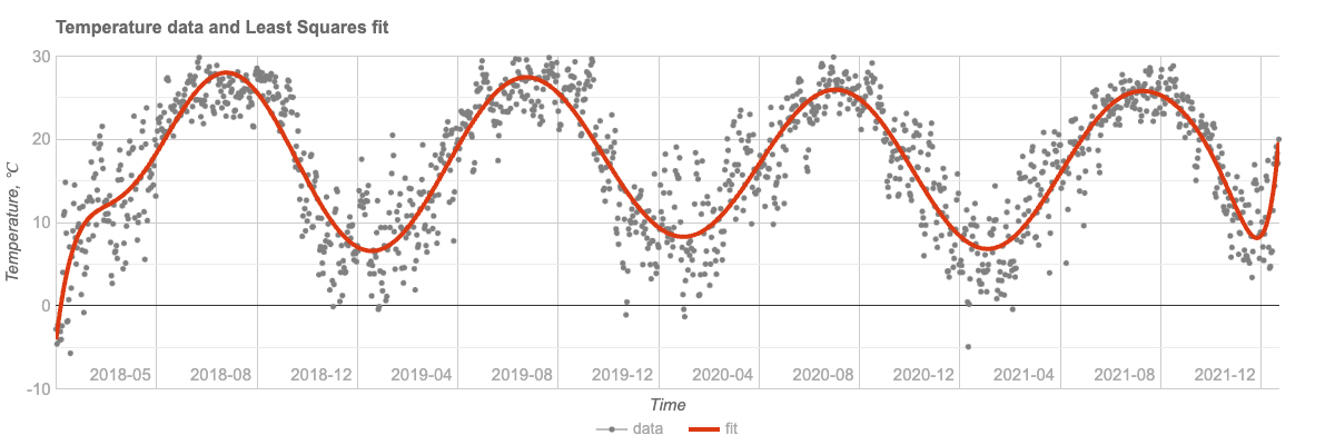
  • A real-life example is demonstrated using weather temperature data. For details, see the section before the last.

Setup

Here are the packages used in this post:

use Math::Polynomial::Chebyshev;
use Math::Fitting;
use Math::Matrix;

use Data::Generators;
use Data::Importers;
use Data::Reshapers;
use Data::Summarizers;
use Data::Translators;
use Data::TypeSystem;

use JavaScript::D3;
use JavaScript::Google::Charts;
use Text::Plot;

use Hash::Merge;

Why use Chebyshev polynomials in fitting?

Chebyshev polynomials provide a powerful and efficient basis for linear regression fitting, particularly when dealing with polynomial approximation and curve fitting. These polynomials, defined recursively, are a sequence of orthogonal polynomials that minimize the problem of Runge’s phenomenon, which is common with high-degree polynomial interpolation.

One of the key advantages of using Chebyshev polynomials in regression is their property of minimizing the maximum error between the fitted curve and the actual data points, known as the minimax property. Because of that property, more stable and accurate approximations are obtained, especially at the boundaries of the interval.

The orthogonality of Chebyshev polynomials with respect to the weight function w(x) = 1/sqrt(1-x^2) on the interval [-1, 1] ensures that the regression coefficients are uncorrelated, which simplifies the computation and enhances numerical stability. Furthermore, Chebyshev polynomials are excellent for approximating functions that are not well-behaved or have rapid oscillations, as they distribute approximation error more evenly across the interval.

Remark: This is one of the reasons Clenshaw-Curtis quadrature was one of the “main” quadrature rules I implemented in Mathematica’s NIntegrate.

Using Chebyshev polynomials into linear regression models allows for a flexible and robust function basis that can adapt to the complexity of the data while maintaining computational efficiency. This makes them particularly suitable for applications requiring high precision and stability, such as in signal processing, numerical analysis, and scientific computing.

Overall, the unique properties of Chebyshev polynomials make them a great regression tool, offering a blend of accuracy, stability, and efficiency.


Chebyshev polynomials computation

This section discusses the computation of Chebyshev polynomials using different methods and their implications on precision.

Computation Granularity

The computation over Chebyshev polynomials is supported on the interval . The recursive and trigonometric methods are compared to understand their impact on the precision of results.

<recursive trigonometric>
==> { .map({ $_ => chebyshev-t(3, 0.3, method => $_) }) }()
# (recursive => -0.792 trigonometric => -0.7920000000000003)

Here polynomial values are computed over a “dense enough” grid:

my $k = 12;
my $method = 'trig'; # 'trig'
my @x = (-1.0, -0.99 ... 1.0);
say '@x.elems : ', @x.elems;

my @data  = @x.map({ [$_, chebyshev-t($k, $_, :$method)]});
my @data1 = chebyshev-t($k, @x);

say deduce-type(@data);
say deduce-type(@data1);
# @x.elems : 201
# Vector(Tuple([Atom((Rat)), Atom((Numeric))]), 201)
# Vector((Any), 201)

Residuals with trigonometric and recursive methods are utilized to assess precision:

sink records-summary(@data.map(*.tail) <<->> @data1)
# +----------------------------------+
# | numerical                        |
# +----------------------------------+
# | 3rd-Qu => 3.3306690738754696e-16 |
# | Max    => 3.4416913763379853e-15 |
# | Median => -3.469446951953614e-18 |
# | 1st-Qu => -6.661338147750939e-16 |
# | Min    => -3.774758283725532e-15 |
# | Mean   => -8.803937402208662e-17 |
# +----------------------------------+

Precision

The exact Chebyshev polynomial values can be computed using FatRat numbers, ensuring high precision in numerical computations.

my $v = chebyshev-t(100, <1/4>.FatRat, method => 'recursive')
# 0.9908630290911637341902191815340830456

The numerator and denominator of the computed result are:

say $v.numerator;
say $v.denominator;
# 2512136227142750476878317151377
# 2535301200456458802993406410752

Plots

This section demonstrates plotting Chebyshev polynomials using Google Charts via the “JavaScript::Google::Charts” package.

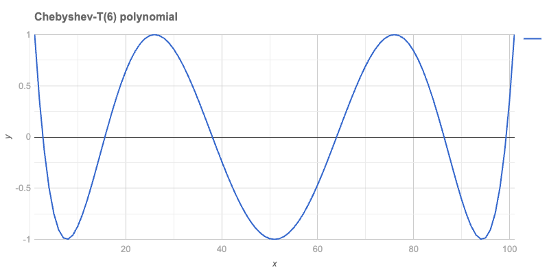
Single Polynomial

A single polynomial can be plotted using a Line chart:

my $n = 6;
my @data = chebyshev-t(6, (-1, -0.98 ... 1).List);
# [1 0.3604845076 -0.1315856097 -0.4953170862 -0.748302037 -0.906688 -0.9852465029 -0.9974401556 -0.9554882683 -0.8704309944 -0.752192 -0.6096396575 -0.4506467656 ...]
#%html
js-google-charts('LineChart', @data, 
    title => "Chebyshev-T($n) polynomial", 
    :$titleTextStyle, :$backgroundColor, :$chartArea, :$hAxis, :$vAxis,
    width => 800, 
    div-id => 'poly1', :$format,
    :png-button)

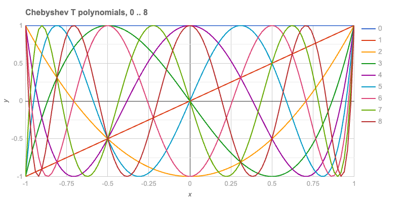
Basis

In fitting, bases of functions are crucial. The first eight Chebyshev-T polynomials are plotted to illustrate this.

my $n = 8;
my @data = (-1, -0.98 ... 1).map: -> $x {
    [x => $x, |(0..$n).map({
         .Str => chebyshev-t($_, $x, :$method)
     })].Hash
}

deduce-type(@data):tally;
# Tuple([Struct([0, 1, 2, 3, 4, 5, 6, 7, 8, x], [Num, Num, Num, Num, Num, Num, Num, Num, Num, Int]) => 1, Struct([0, 1, 2, 3, 4, 5, 6, 7, 8, x], [Num, Num, Num, Num, Num, Num, Num, Num, Num, Rat]) => 100], 101)

The plot with all eight functions is shown below:

#%html
js-google-charts('LineChart', @data,
    column-names => ['x', |(0..$n)».Str],
    title => "Chebyshev T polynomials, 0 .. $n",
    :$titleTextStyle,
    width => 800, 
    height => 400,
    :$backgroundColor, :$hAxis, :$vAxis,
    legend => merge-hash($legend, %(position => 'right')),
    chartArea => merge-hash($chartArea, %(right => 100)),
    format => 'html', 
    div-id => "cheb$n",
    :$format,
    :png-button)

Text Plot

Text plots provide a reliable method for visualizing data anywhere! The data is converted into a long form to facilitate plotting using “Text::Plot”.

my @dataLong = to-long-format(@data, <x>).sort(*<Variable x>);
deduce-type(@dataLong):tally
# Tuple([Struct([Value, Variable, x], [Num, Str, Int]) => 9, Struct([Value, Variable, x], [Num, Str, Rat]) => 900], 909)

A sample of the data is provided:

@dataLong.pick(8)
  ==> {.sort(*<Variable x>)}()
  ==> to-html(field-names => <Variable x Value>)
VariablexValue
1-0.18-0.18
3-0.440.979264
30.66-0.830016
6-0.92-0.7483020369919988
60.560.9111532625919998
8-0.60.42197247999999865
80.080.8016867058843643
80.660.8694861561561088

The text plot is presented here:

my @chebInds = 1, 2, 3, 4;
my @dataLong3 = @dataLong.grep({
    $_<Variable>.Int ∈ @chebInds
}).classify(*<Variable>).map({
    .key => .value.map(*<x Value>).Array
}).sort(*.key)».value;

text-list-plot(@dataLong3,
  width => 100,
  height => 25,
  title => "Chebyshev T polynomials, 0 .. $n",
  x-label => (@chebInds >>~>> ' : ' Z~ <* □ ▽ ❍>).join(', ')
);
# Chebyshev T polynomials, 0 .. 8                                   
# +----+---------------------+---------------------+---------------------+---------------------+-----+      
# |                                                                                                  |      
# +    ❍                  ▽▽▽▽▽▽▽▽               ❍❍❍❍❍❍                                       *❍     +  1.00
# |     □              ▽▽▽        ▽▽▽         ❍❍❍      ❍❍❍                               ***** □     |      
# |      □□          ▽▽              ▽▽     ❍❍            ❍                          ****    □□▽     |      
# |     ❍  □        ▽▽                 ▽▽▽ ❍               ❍❍                   *****       □ ▽❍     |      
# |         □      ▽                     ❍❍▽                 ❍❍             *****          □         |      
# +          □□   ▽                     ❍  ▽▽                  ❍        ****             □□  ▽       +  0.50
# |      ❍    □  ▽                     ❍     ▽                  ❍  *****                □   ▽ ❍      |      
# |            ▽▽                    ❍❍       ▽▽               **❍*                    □             |      
# |       ❍      □□                 ❍           ▽▽        *****   ❍                  □□    ▽ ❍       |      
# |           ▽    □                ❍             ▽▽  *****        ❍                □     ▽          |      
# +        ❍  ▽     □□             ❍              *▽**              ❍             □□     ▽  ❍        +  0.00
# |          ▽       □□           ❍          *****  ▽▽               ❍          □□                   |      
# |         ❍          □□        ❍       ****         ▽▽              ❍        □□       ▽  ❍         |      
# |                      □□    ❍❍   *****               ▽              ❍❍    □□        ▽             |      
# |        ▽ ❍             □□ ❍ *****                    ▽▽              ❍ □□         ▽▽  ❍          |      
# +       ▽   ❍             *❍□*                          ▽▽             ❍□          ▽   ❍           + -0.50
# |                    ***** ❍ □□□                          ▽▽        □□□ ❍         ▽                |      
# |      ▽    ❍    ****    ❍❍     □□□                         ▽▽   □□□     ❍❍     ▽▽    ❍            |      
# |     ▽     *❍❍**      ❍❍         □□□□                        ▽▽□          ❍❍ ▽▽     ❍             |      
# |       *****  ❍     ❍❍               □□□□□             □□□□□□  ▽▽▽▽        ▽❍❍     ❍              |      
# +    ▽**        ❍❍❍❍❍                      □□□□□□□□□□□□□□           ▽▽▽▽▽▽▽▽  ❍❍❍❍❍❍               + -1.00
# |                                                                                                  |      
# +----+---------------------+---------------------+---------------------+---------------------+-----+      
#      -1.00                 -0.50                 0.00                  0.50                  1.00         
#                                      1 : *, 2 : □, 3 : ▽, 4 : ❍

Fitting

This section presents the generation of “measurements data” with noise and the fitting process using a function basis.

my @temptimelist = 0.1, 0.2 ... 20;
my @tempvaluelist = @temptimelist.map({
    sin($_) / $_
}) Z+ (1..200).map({
    (3.rand - 1.5) * 0.02
});
my @data1 = @temptimelist Z @tempvaluelist;
@data1 = @data1.deepmap({ .Num });

deduce-type(@data1)
# Vector(Vector(Atom((Numeric)), 2), 200)

Rescaling of x-coordinates is performed as follows:

my @data2 = @data1.map({ my @a = $_.clone; @a[0] = @a[0] / max(@temptimelist); @a });

deduce-type(@data2)
# Vector(Vector(Atom((Numeric)), 2), 200)

A summary of the data is provided:

sink records-summary(@data2)
# +------------------+----------------------------------+
# | 0                | 1                                |
# +------------------+----------------------------------+
# | Min    => 0.005  | Min    => -0.23878758770507946   |
# | 1st-Qu => 0.2525 | 1st-Qu => -0.053476022454404415  |
# | Mean   => 0.5025 | Mean   => 0.07323149609113122    |
# | Median => 0.5025 | Median => -0.0025316517415275193 |
# | 3rd-Qu => 0.7525 | 3rd-Qu => 0.07666085422352723    |
# | Max    => 1      | Max    => 1.0071290191857256     |
# +------------------+----------------------------------+

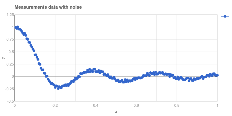
The data is plotted below:

#% html
js-google-charts("Scatter", @data2, 
    title => 'Measurements data with noise',
    :$backgroundColor, :$hAxis, :$vAxis,
    :$titleTextStyle, :$chartArea,
    width => 800, 
    div-id => 'data', :$format,
    :png-button)

A function to rescale from [0,1] to [-1, 1] is defined:

my &rescale = { ($_ - 0.5) * 2 };

The basis functions are listed:

my @basis = (^16).map: { chebyshev-t($_) o &rescale }
@basis.elems
# 16

Remark: The function composition operator o is utilized above. The argument is rescaled before computing the Chebyshev polynomial value.

A linear model fit is computed using these functions:

my &lm = linear-model-fit(@data2, :@basis)
# Math::Fitting::FittedModel(type => linear, data => (200, 2), response-index => 1, basis => 16)

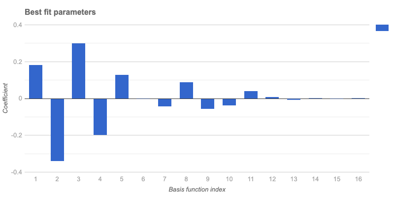
The best fit parameters are:

&lm('BestFitParameters')
# [0.18012514065989924 -0.3439467053791086 0.29469719162086117 -0.20515007850826206 0.12074121627488964 -0.003435776130307378 -0.047297896072549465 0.08663571434303828 -0.058165484141402886 -0.03933300920226471 0.03907623399167609 0.0015109810557268964 -0.011525135506292928 -0.0045136819929066 0.0021477767328720826 -0.004624145810439574]

The plot of these parameters is shown:

#% html
js-google-charts("Bar", &lm('BestFitParameters'), 
    :!horizontal,
    title => 'Best fit parameters',
    :$backgroundColor, 
    hAxis => merge-hash($hAxis, {title => 'Basis function index'}), 
    vAxis => merge-hash($hAxis, {title => 'Coefficient'}), 
    :``titleTextStyle, :``chartArea,
    width => 800, 
    div-id => 'bestFitParams', :$format,
    :png-button)

It is observed from the plot that using more than 12 basis functions does not improve the fit, as coefficients beyond the 12th index are very small.

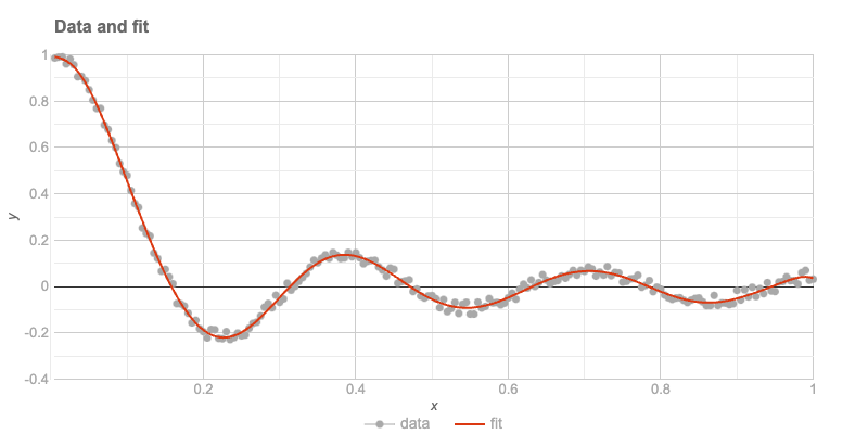
The data and the fit are plotted after preparing the plot data:

my @fit = @data2.map(*.head)».&lm;
my @plotData = transpose([@data2.map(*.head).Array, @data2.map(*.tail).Array, @fit]);
@plotData = @plotData.map({ <x data fit>.Array Z=> $_.Array })».Hash;

deduce-type(@plotData)
# Vector(Assoc(Atom((Str)), Atom((Numeric)), 3), 200)

The plot is presented here:

#% html
js-google-charts('ComboChart', 
    @plotData, 
    title => 'Data and fit',
    column-names => <x data fit>,
    :``backgroundColor, :``titleTextStyle :``hAxis, :``vAxis,
    seriesType => 'scatter',
    series => {
        0 => {type => 'scatter', pointSize => 2, opacity => 0.1, color => 'Gray'},
        1 => {type => 'line'}
    },
    legend => merge-hash($legend, %(position => 'bottom')),
    :$chartArea,
    width => 800, 
    div-id => 'fit1', :$format,
    :png-button)

The residuals of the last fit are computed:

sink records-summary( (@fit <<->> @data2.map(*.tail))».abs )
# +----------------------------------+
# | numerical                        |
# +----------------------------------+
# | Max    => 0.03470224056776856    |
# | Median => 0.0136727625440904     |
# | Min    => 0.00011187750898611348 |
# | 1st-Qu => 0.006365201141942046   |
# | Mean   => 0.01363628423382272    |
# | 3rd-Qu => 0.019937969354319008   |
# +----------------------------------+

Condition Number

The Ordinary Least Squares (OLS) fit is computed using the formula:

β=(t(X).X)^(-1).t(X).y, where t(X) is the transpose of X.

The condition number of the “normal matrix” (or “Gram matrix”) t(X).X is examined. The design matrix is obtained first:

my @a = &lm.design-matrix();
my $X = Math::Matrix.new(@a);
$X.size
# (200 16)

The Gram matrix is:

my $g = $X.transposed.dot-product($X);
$g.size
# (16 16)

The condition number of this matrix is:

$g.condition
# 88.55110861577737

It is concluded that the design matrix is suitable for use.

Remark: For a system of linear equations in matrix form Ax=b, the condition number of A, k(A), is defined as the maximum ratio of the relative error in x to the relative error in b.

Remark: Typically, if the condition number is k(A)=10^d, up to d digits of accuracy may be lost in addition to any loss caused by the numerical method (due to precision issues in arithmetic calculations).

Remark: A very “Raku-way” to define an ill-conditioned matrix is as “almost not of full rank” or “almost as if its inverse does not exist.”


Temperature Data

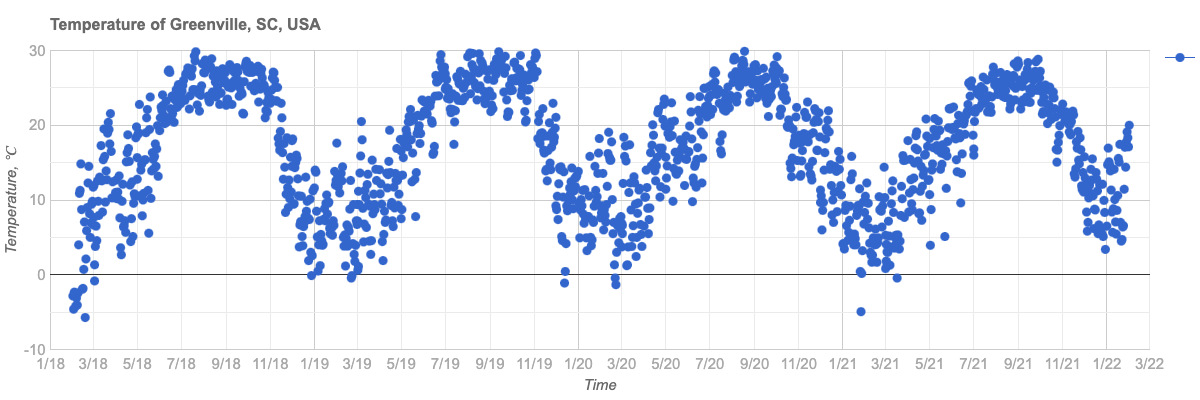
The entire workflow is repeated with real-life data, specifically weather temperature data for four consecutive years in Greenville, South Carolina, USA. This location is where the Perl and Raku Conference 2025 will be held.

The time series data is ingested:

my $url = 'https://raw.githubusercontent.com/antononcube/RakuForPrediction-blog/refs/heads/main/Data/dsTemperature-Greenville-SC-USA.csv';

my @dsTemperature = data-import($url, headers => 'auto');
@dsTemperature = @dsTemperature.deepmap({ ``_ ~~ / ^ \d+ '-' / ?? DateTime.new(``_) !! $_.Num });
deduce-type(@dsTemperature)
# Vector(Struct([AbsoluteTime, Date, Temperature], [Num, DateTime, Num]), 1462)

A summary of the data is shown:

sink records-summary(
  @dsTemperature, field-names => <Date AbsoluteTime Temperature>
);
# +--------------------------------+----------------------+------------------------------+
# | Date                           | AbsoluteTime         | Temperature                  |
# +--------------------------------+----------------------+------------------------------+
# | Min    => 2018-01-01T00:00:37Z | Min    => 3723753600 | Min    => -5.72              |
# | 1st-Qu => 2019-01-01T00:00:37Z | 1st-Qu => 3755289600 | 1st-Qu => 10.5               |
# | Mean   => 2020-01-01T12:00:37Z | Mean   => 3786868800 | Mean   => 17.053549931600518 |
# | Median => 2020-01-01T12:00:37Z | Median => 3786868800 | Median => 17.94              |
# | 3rd-Qu => 2021-01-01T00:00:37Z | 3rd-Qu => 3818448000 | 3rd-Qu => 24.11              |
# | Max    => 2022-01-01T00:00:37Z | Max    => 3849984000 | Max    => 29.89              |
# +--------------------------------+----------------------+------------------------------+

The plot of the data is provided:

#% html
js-google-charts("Scatter", @dsTemperature.map(*<Date Temperature>), 
    title => 'Temperature of Greenville, SC, USA',
    :$backgroundColor,
    hAxis => merge-hash($hAxis, {title => 'Time', format => 'M/yy'}), 
    vAxis => merge-hash($hAxis, {title => 'Temperature, ℃'}), 
    :``titleTextStyle, :``chartArea,
    width => 1200, 
    height => 400, 
    div-id => 'tempData', :$format,
    :png-button)

The fit is performed with rescaling:

my (``min, ``max) = @dsTemperature.map(*<AbsoluteTime>).Array.&{
  (.min, .max)
}();
# (3723753600 3849984000)
my &rescale-time = {
    -(``max + ``min) / (``max - ``min) + (2 * ``_) / (``max - $min)
}
my @basis = (^16).map({ chebyshev-t($_) o &rescale-time });
@basis.elems
# 16
my &lm-temp = linear-model-fit(
  @dsTemperature.map(*<AbsoluteTime Temperature>), :@basis
);
# Math::Fitting::FittedModel(type => linear, data => (1462, 2), response-index => 1, basis => 16)

The plot of the time series and the fit is presented:

my @fit = @dsTemperature.map(*<AbsoluteTime>)».&lm-temp;
my @plotData = transpose([
  @dsTemperature.map(*<AbsoluteTime>).Array,
  @dsTemperature.map(*<Temperature>).Array,
  @fit
]);
@plotData = @plotData.map({ <x data fit>.Array Z=> $_.Array })».Hash;

deduce-type(@plotData)
# Vector(Assoc(Atom((Str)), Atom((Numeric)), 3), 1462)
#% html

my @ticks = @dsTemperature.map({
    %( v => ``_<AbsoluteTime>, f => ``_<Date>.Str.substr(^7))
})».Hash[0, 120 ... *];

js-google-charts('ComboChart', 
    @plotData,
    title => 'Temperature data and Least Squares fit',
    column-names => <x data fit>,
    :``backgroundColor, :``titleTextStyle,
    hAxis => merge-hash($hAxis, {title => 'Time', :@ticks, textPosition => 'in'}), 
    vAxis => merge-hash($hAxis, {title => 'Temperature, ℃'}), 
    seriesType => 'scatter',
    series => {
        0 => {type => 'scatter', pointSize => 3, opacity => 0.1, color => 'Gray'},
        1 => {type => 'line', lineWidth => 4}
    },
    legend => merge-hash($legend, %(position => 'bottom')),
    :$chartArea,
    width => 1200, 
    height => 400, 
    div-id => 'tempDataFit', :$format,
    :png-button)

Future Plans

The current capabilities of Raku in performing regression analysis for both educational and practical purposes have been demonstrated.

Future plans include implementing computational frameworks for Quantile Regression in Raku. Additionally, the workflow code in this post can be generated using Large Language Models (LLMs), which will be explored soon.

Day 16 – Revision gating in Rakudo core

The motivation

One of the Rakudo features I worked on this year was to resolve an annoyance related to the Array.splice method. As reported in a GitHub issue called Array.splice insists on flattening itself:

my @map = [[11, 12], [31,32]];
my @newrow = [21, 22];
@map.splice(1, 0, @newrow);

# Expected
[
  [11, 12],
  [21, 22],
  [31, 32]
]

# Actual
[
  [11, 12],
  21,
  22,
  [31, 32]
]

The author of the ticket tried all sorts of mechanisms to inform splice that the @newrow array should be inserted as a single element.

@map.splice(1, 0, [[[[@newrow]]]]);
@map.splice(1, 0, $@newrow);

But unfortunately these efforts were to no avail.

The “real” way to achieve the semantics the user wanted would be:

@map.splice(1, 0, [$@newrow,])

I’m not sure if hanging-commas-to-declare-single-element-lists ever genuinely did anything worthy to earn the exact volume of my distaste for them. Nevertheless I viscerally react when I see this syntax.

Not only this, but in the recent history prior to my reading this issue on Github, I had been personally annoyed by this exact issue in splice .

Clearly it was time to take this thing head-on.

This hubristic impulse led me down a rabbit hole from which it took three pull requests and a handful of months in order to extract myself.

A solution to the splice problem

I’m going to avoid wading too far into the depths of the solution — the is item trait — I crafted to resolve the above issue, as that would be a lengthy post all on its own.

However, it is worth showing a bit of how it works:

multi combine (@a, $b) { 
    [|@a,  [@a[0][0],$b]] 
}
​
multi combine (@a is item, $b) {
    # the non-itemized array returned here will match
    # the "regular" @a signature
    [@a, [@a[0], $b]]
}
​
​
multi combine ($a, $b) { 
    # The itemized array returned here will match
    # the signature containing `@a is item`
    $[$a, $b]
}
​
(reduce &combine, 1..5).raku.say;
# [[1, 2], [1, 3], [1, 4], [1, 5]]

Or, more directly using Array.splice:

use v6.e.PREVIEW; # THIS PART IS CRUCIAL!
​
my @presents = [<
  pear-tree-partridge turtle-dove french-hen calling-bird 
  golden-rings eggy-goose swimmy-swan milky-maid dancey-lady 
  leapy-lord pipey-piper drummy-drummer
>];
​
multi sub present-supplier(Int $day) {
  [ @presents[$day] xx $day+1 ]
}
​
my @christmas-presents-flat;
for ^12 -> $nth-day {
# if $nth-day == 0 {
#   @christmas-presents-flat[$nth-day] = present-supplier($nth-day)[0];
#  } 
#  else {
    @christmas-presents-flat.splice: *, 0, present-supplier($nth-day);
#  }
}
​
use PrettyDump;
pd @christmas-presents-flat;
# Array=[
#   "turtle-dove",
#   "french-hen",
#   "french-hen",
#   ...
#   "drummy-drummer",
#   "drummy-drummer"
# ]
​
multi sub present-supplier(Int $day, :$itemize!) {
  $[ @presents[$day] xx $day+1 ]
}
​
my @christmas-presents-segmented;
for ^12 -> $nth-day {
  @christmas-presents-segmented.splice: *, 0, present-supplier($nth-day, :itemize);
}
​
pd @christmas-presents-segmented;
# Array=[
#   Array=[
#       "pear-tree-partridge"
#   ],
#   Array=[
#       "turtle-dove",
#       "turtle-dove"
#   ],
#   Array=[
#       "french-hen",
#       "french-hen"
#   ],
#   ...
# ]

This new functionality was made possible by adding candidates to Array.splice which utilized the is item trait to dispatch a nested form of the array to the primary Array.splice candidate. (There are a lot of Array.splice candidates, but they all eventually funnel into an optimized candidate.)

Here is an example candidate, and in fact the one we are using in our examples:

multi method splice(Array:D:
  Callable:D $offset, Int:D $size, @new is item
--> Array:D) is revision-gated("6.e") {
    self.splice($offset(self.elems),$size,[$@new])
}

So here we are passing along the @new array as the single itemized element in a wrapper array. When this gets to Array.splice‘s handler candidate, it will flatten the wrapper array and receive @new as a single item to be spliced in.

However, in doing so I had now changed the base behavior of Array.splice. Any code that was working as expected with itemized array arguments would break.

So, how could we introduce these new semantics into Rakudo without breaking existing code?

Therein, my friends, lay the rabbit hole at the bottom of the rabbit hole.

Enter revision gating

After some consultation on #raku-dev, I started hacking on a mechanism to mark multi candidates as “gated” to a specific revision baseline. For the @new is item candidates in Array.splice , these would be gated to language revisions 6.e and above.

This is done through a combination of features that run pretty deeply into Rakudo’s CORE.setting:

  1. A new is trait needed to be created.
  2. The Routine class needed to know how to become revision gated.
    1. These changes to Routine need to be supported by additions to BOOTSTRAP.nqp
  3. The dispatcher needed to be made aware of revision gating and capable of handling it.

Adding the is revision-gated trait declaration

In my opinion traits are deeply cool. I often miss them when I’m programming in other languages. It’s a way to sugar over what would otherwise be some gnarly-ish metaprogramming code. Underneath, it remains said gnarly-ish metaprogramming — but it doesn’t clutter up your declaration locations. In some sense, traits are sort of a way to make metaprogramming look as safe as it actually is.

Here’s the declaration I used for is revision-gated:

multi sub trait_mod:<is>(Routine:D $r, Str :$revision-gated!) {
    my $chars := nqp::chars($revision-gated);
    my $internal-revision :=
      1 + nqp::ord($revision-gated, $chars - 1) - nqp::ord("c");
    $r.set-revision-gated;
    $r.^mixin(role is-revision-gated[$revision] {
        method REQUIRED-REVISION(--> Int) { $revision }
    }.^parameterize($internal-revision));
}

I don’t think anyone would want to look at this very often, so having it in a trait is perfect. Many traits make use of ^mixin to include a role, which can be anonymous or named (as we have here, to be able to parameterize it).

Due to the earliness where it should be possible to use this trait in the Rakudo setting, we have to do the parameterization of the role via ^parameterize rather than passing it in as a simple lexical (thanks to nine++ for devising the final incantation).

The ultimate impact of the trait is two-fold:

  1. It flips a bit field in the routine object to mark it as having revision gating ($r.set-revision-gated).
  2. It installs a REQUIRED-REVISION method that returns the minimum required revision as an Int.

Bootstrap concerns

Since the call to set-revision-gated is happening very early on in the setup of the Routine object, that method needs to be defined and made available through our bootstrap.c/BOOTSTRAP.nqp module, rather than as a method defined in Routine.rakumod.

Routine.HOW.add_method(Routine, 'set-revision-gated',
  nqp::getstaticcode(sub ($self) {
      $self.set_flag(0x08);
  })
);

We also need a method for checking this flag:

Routine.HOW.add_method(Routine, 'revision-gated',
  nqp::getstaticcode(sub ($self) {
     $self.get_flag(0x08);
  })
);

Also, we want to include the required revision for the candidate in the hash of “candidate info” that is stored in a field of the Routine object and which the dispatcher will eventually be using in favor of having to call methods on candidate objects (a much more costly affair):

Routine.HOW.add_method(Routine, '!create_dispatch_info',
  nqp::getstaticcode(sub ($self) {
      $self := nqp::decont($self);
      ...
      if $self.revision-gated {
          nqp::bindkey(%info, 'required_revision', $self.REQUIRED-REVISION);
      }
      ...
      nqp::bindattr($self, Routine, '$!dispatch_info', %info)
  })
);

With that we are mostly through with fiddling with the bootstrap, except in the case of the JVM, which also installs a private method onto Routine called !filter-revision-gated-candidates that will be used by the “old” dispatcher code. We will see the contents of this routine next, but in the context of MoarVM’s dispatcher, and otherwise won’t be talking about the JVM implementation here beyond mentioning that it is at feature parity with MoarVM.

Dispatching to specific revisions

The dispatcher code was recently revised and optimized. I had gotten somewhat familiar with it while adding is item, so I knew a bit of how to poke at it.

From a bird’s eye view, when a multi is called, the dispatcher receives the proto candidate and an argument capture. The dispatcher asks the proto for a list of %dispatcher_info hashes that are then whittled down to the subset of hashes that are suitable for the provided argument capture.

So then, “all” I needed to do was filter out any candidates not meeting the language revision criteria (if any) from the list of candidate hashes before that list is sent to the whittling function.

Here’s the logic that checks if the proto mentions any revision gating:

my @candidates := nqp::bitand_i(
  nqp::getattr_i($target, Routine, '$!flags'), 0x08
) ?? (my $caller-revision := nqp::getlexcaller('$?LANGUAGE-REVISION') // 1) 
       && $target.REQUIRED-REVISION <= $caller-revision
    ?? multi-filter-revision-gated-candidates($target, $caller-revision)
    !! []
  !! $target.dispatch_order;

So, if there’s no bit flipped in $!flag to indicate revision gating, we simply return $target.dispatch_order.

Otherwise, we pull $?LANGUAGE-REVISION from the lexpad (it gets installed at the top-level of every compunit) and we compare it against $target.REQUIRED-REVISION (where $target is the proto). If $target has a higher revision requirement than the $caller-revision than none of its multis will likewise have their requirements met. So in this case we set @candidates an empty list, which bubbles up to a dispatch error almost immediately.

In the more common case where the proto‘s revision requirement is met, we call multi-filter-revision-gated-candidates:

sub multi-filter-revision-gated-candidates($proto, $caller-revision) {
  my @candidates := $proto.dispatch_order;

  my int $idx := 0;
  my int $allowed-idx := 0;
  my @allowed-candidates;
  my %gated-candidates;
  while $idx < nqp::elems(@candidates) {
      my $candidate := nqp::atpos(@candidates, $idx++);

      unless nqp::isconcrete($candidate) {
          nqp::push(@allowed-candidates, $candidate);
          $allowed-idx++;
          next;
      }

      my $required-revision := nqp::atkey($candidate, 'required_revision');
      my $is-revision-specified := nqp::isconcrete($required-revision);
      if !$is-revision-specified || $required-revision <= $caller-revision {
          if (nqp::existskey($candidate, 'signature')) && $is-revision-specified {
              my $signature := nqp::atkey($candidate, 'signature').raku;
              if nqp::existskey(%gated-candidates, $signature) {
                  # this is what was set as the $allowed-idx in a previous run
                  my $candidate-idx := nqp::atkey(%gated-candidates, $signature);
                  my $last-seen-revision := nqp::atkey(
                      nqp::atpos(@allowed-candidates, $candidate-idx),
                      'required_revision'
                  );

                  if $last-seen-revision < $required-revision {
                      nqp::bindkey(%gated-candidates, $signature, $candidate-idx);
                      nqp::bindpos(@allowed-candidates, $candidate-idx, $candidate);
                      # Do *not* bump $allowed-idx here
                  }
              } else {
                  nqp::push(@allowed-candidates, $candidate);
                  nqp::bindkey(%gated-candidates, $signature, $allowed-idx++);
              }
          } else {
              nqp::push(@allowed-candidates, $candidate);
              $allowed-idx++;
          }
      }
  }

  @allowed-candidates
}

A primary consideration here is that $proto.dispatch_order returns an organized list of candidate info hashes. This means we need to preserve the ordering while kicking out any inadequate candidates.

Initially routine covered fewer edge cases, and thus was slightly simpler. But since revision gating should also be able to replace multis that have the same signature but where a change of functionality is desired, I introduced the %gated-candidates hash to track minimum revision gated versions for candidates of the same signature.

This has the functional effect of allowing for the introduction of ceilings and floors for otherwise-matching candidates. This is probably best shown in an example:

How to use is revision-gated

(Please note: this evolution did not land in time for the 2024.12, so you will need to wait for 2025.01 or build Rakudo from source to use revision gating of candidates with equivalent signatures.)

my $to-eval = q:to/END/;
​
proto sub gated(|) is revision-gated("6.c") {*}
multi sub gated(Int $x) is revision-gated("6.c") { print "6.c ($x)" }
multi sub gated(Int $x) is revision-gated("6.d") { print "6.d ({$x+1})" }
multi sub gated(Int $x) is revision-gated("6.e") { print "6.e ({$x+2})" }
​
gated(6);
​
END
​
is-run 'use v6.c;' ~ $to-eval,
  :out("6.c (6)"),
  q|is revision-gated("6.c") candidate called for 'use v6.c;'|;

is-run 'use v6.d;' ~ $to-eval,
  :out("6.d (7)"),
  q|is revision-gated("6.d") candidate called for 'use v6.d;'|;

is-run 'use v6.e.PREVIEW;' ~ $to-eval,
  :out("6.e (8)"),
  q|is revision-gated("6.e") candidate called for 'use v6.e;'|;

(Note: is-run is provided by Test::Helpers which is not currently provided outside of Rakudo’s test suite.)

Here each candidate has a clear floor and ceiling: each can only run on a single language revision.

However, if we removed the 6.d candidate, the “floor” of the 6.c candidate would be 6.c and the “ceiling” would be 6.d, as a replacement is then provided in 6.e. These “floor”/”ceiling” values are implicit and contextual.

Required ingredients

Revision gating requires the following to be in place in order to work:

  • The proto must specify the minimum revision for all of it’s candidates.
    • proto sub gated(|) is revision-gated("6.c") {*}
  • The new candidate must specify the revision of it’s introduction.
    • multi sub gated(Int $x) is revision-gated("6.e")

However, as mentioned above, it is important to follow this additional rule:

  • If the new candidate replaces an existing candidate of the same signature, the multi candidate to be replaced must set it’s own minimum revision.
    • multi sub gated(Int $x) is revision-gated("6.c")

Eventually the requirement of specifying a minimum revision for the proto may be removed but at the moment there were bootstrapping/circularity issues in play that prevented a minimum revision to be automatically installed.

Gate it and upgrade it!

I hope this helps in shedding some light on the revision-gated trait and unlocks some opportunities for code in both Rakudo core and in user space to evolve their semantics safely and effectively.

Post Scriptum

While implementing this feature, I was mostly oblivious to some long-running discussions about how to achieve the evolution of semantics across language revisions. Later I found this problem-solving ticket, which almost certainly represents only the very tip of the iceberg.

But I only found that ticket because, after merging the initial version, nine informed me of the following:

nine ab5tract: you do realize that you have finally implemented something we have only talked about for 6 or 7 years? Thanks a lot!

To which I replied:

ab5tract kind of reminds me of my trainer at the gym.. he takes care not to tell me how much weight I’m lifting until after I’m done lifting it 🙂

It’s been a great year with some heavy lifting in core and so I want to say a mega-large thank you to all the folks in #raku and #raku-dev who have managed to put up with my ups-and-downs this year. It means a lot to to me, being in the presence of such a diversely talented crowd.

Day 15 – Matching Maps

Lizzybel was again walking through the corridors of North Pole Grand Central and was stopped by Nanunanu, one of the IT elves, with a face a little paler than usual. “So what is the problem?” Lizzybel asked.

Nanunanu took a deep breath and started: “…so we have built this sorta in-memory database in a Raku hash, like a key/value store. But now we need to be able to do regex matching on the keys, and Raku hashes don’t do that by themselves. And looping over the keys and matching them one at a time is just taking too long. And now we’re looking at a deadline, and the department elf is getting all upset, and the holidays are coming nearer and nearer, and we don’t know what to do”. Actually, Nanunanu’s stream of consciousness went on for a little while more, but you all get the picture!

When Nanunanu drew a breath again, Lizzybel asked: “Well, that’s quite a pickle you got your and your team in, have you tried hypering?”. Nanunanu looked perplexed. “Hypering? Isn’t that like super complicated? But no, we haven’t tried that” while getting a little hope that there would be a way out of this stressful situation.

“Ok, let’s do some testing”, Lizzybel said while she grabbed her notebook. “I assume that this hash is actually mostly static?” she asked, and Nanunanu nodded. Lizzybel then started to write some code:

my %h is Map = "words".IO.lines.map: { $_ => $_ }
say "Found %h.elems() words";
{
    LEAVE say now - ENTER now;
    say %h.keys.grep: { / foo $ / }
}

Showing this to Nanunanu she said: “I always keep a local copy of the ‘words’ file in my home directory, just for these things.”

And then continued: “So the first line just creates a Map with all the words. Then it shows how many words we have. The LEAVE phaser and the ENTER phaser are used to give us the time that was spent in the lookup. And the last line in the block does the actual work, grepping through the keys of this Map looking for any keys that end with foo.”

Lizzybel then ran the program, and it said:

Found 235976 words
(foo mafoo)
0.446319075

“Ok, that’s a good beginning” said Nanunanu with the color starting to return to their face.

“Yes, it is, but this can be made faster, because a bare / foo $ / is just doing too much work if you just want to see whether it matched. For that, you can also use .contains“:

my %h is Map = "words".IO.lines.map: { $_ => $_ }
{ 
    LEAVE say now - ENTER now;
    say %h.keys.grep(*.contains(/ foo $ /);
}   

which showed:

(mafoo foo)
0.356022428

“The trick there is that .contains does not need to create a relatively expensive Match for each check, it just needs to return True or False“, Lizzybel explained. “And that’s already about 25% faster” said Nanunanu, showing off their amazing math skills.

“Now, if you have more than one CPU, you can use all of the other ones as well, which might make things faster, but will cost more energy because of overhead of splitting up the work over multiple CPUs and then gathering the results again. And you only need to add .hyper at the right place” Lizzybel said while moving the cursor to the right place and entering just that.

my %h is Map = "words".IO.lines.map: { $_ => $_ }
{ 
    LEAVE say now - ENTER now;
    say %h.keys.hyper.grep(*.contains(/ foo $ /);
}   

Running that program showed:

(mafoo foo)
0.170500436

“WOW” shouted Nanunanu, “that’s more than twice as fast!”. “Yup”, Lizzybel agreed, “but it can get even better. Because there’s this module called Map::Match“, and off she went with:

$ zef install Map::Match
===> Searching for: Map::Match
===> Staging Map::Match:ver<0.0.8>:auth<zef:lizmat>
===> Staging [OK] for Map::Match:ver<0.0.8>:auth<zef:lizmat>
===> Testing: Map::Match:ver<0.0.8>:auth<zef:lizmat>
===> Testing [OK] for Map::Match:ver<0.0.8>:auth<zef:lizmat>
===> Installing: Map::Match:ver<0.0.8>:auth<zef:lizmat>

“That’s a special version of Map where the keys can be regular expressions. Let’s see how that works out” Lizzybel continued, smiling.

use Map::Match;
my %h is Map::Match = "words".IO.lines.map(* => 1);
{
    LEAVE say now - ENTER now;
    say (%h{/ foo $ /}:k);
}

which showed:

(mafoo foo)
0.063553282

“Ooh, that’s cool: still 2.5x as fast as the hypered version”, Nanunanu shouted out while clapping their hands. “Yes it is” Lizzybel thought, “that was a nice piece of work I did there. And it didn’t even needed hypering under the hood, just a little NQP cheating”.

Nanunanu quickly went back to their team in the knowledge that they might be able to make things up to 7 times faster. “Thanks Lizzybel”, they said while running through the corridors of North Pole Grand Central.

And all was well.

Day 14 – Playing around with the new documentation components

After living with RakuDoc v2 for over a year, some things become normal that surprise others when I explain them. Here are a few things I do when documenting my software.

1. Shoving stuff down the file

There are a couple of items needed in a changing document that should be easily managed, probably at the top of the file, but which are best rendered at the bottom. This is easily done using a semantic block with :hidden. Suppose at the top of the document we have the following

=TITLE An important document
=begin AUTHORS :hidden
=item A. Writer
=item A.N. Other
=end AUTHORS

The TITLE contents (An important document) will be rendered, but the contents of the AUTHORS semantic block will not.

A note to those unaccustomed to RakuDoc: if a block name starts immediately after an =, then the contents of the block start on the same line, and end when the first blank line is encountered.

Since AUTHORS is preceded by =begin, the rest of the first line is metadata and the contents start on the next line until the =end AUTHORS line.

The contents of a semantic block, which is identified because the name is all caps, are processed and stored.

The :hidden prevents the contents from being immediately added to the output. Later, eg. at the bottom of the file, we can indicate where the processed string is added to the output using a =place block, for example,

=place semantic:AUTHORS :caption<Credits>

Here =place seems to be a block, but it is considered to be a directive. A directive does not have a =for or =begin form, and can be followed by metadata. In this case, ‘semantic:’ indicates where the place block is getting its data, while :caption contains a string that is used to add the block to the Table of Contents, and to act as a heading in the flow of the text.

=place can be used to include images (online or local), other rakudoc files, and several other types of data. By the way, it is possible to =place data from the current source file that has not yet been processed. Thus, it is possible to have a =place semantic:SOMENAME before specifying =SOMENAME.

2. Configuration

When writing this source in RakuDoc, which will be included at the end of the article, I will be including a number of examples as code.

RakuDoc allows for code to included without explicitly requiring a =begin code / =end code sequence. All that is needed is to indent the text in a block without any blank lines.

A code block can be marked with the metadata option :lang to indicate which computer language is contained in the block, for example so that a syntax highlighter can be used. A code block without :lang is considered by default to be Raku.

An implicit code block has nothing to ‘hang’ a :lang on, but I want for all the implicit code blocks in this article to be :lang<RakuDoc>. I can do this using the =config directive, eg.

=config code :lang<RakuDoc>

The statement means that all code blocks, which also includes all implicit code blocks, are by default :lang<RakuDoc>.

More generally, a config directive expects a block name followed by one or more metadata options. Then by default each successive block with that name will have that metadata option set to the value in the config directive. The scope of the config directive can be controlled, as explained in the specification.

3. Numbering

One of the really irritating aspects I found in RakuDoc v1 (POD6) was that numbered items or headings was not possible. As you can see this has been overcome. Up to four levels of numbering are automatically supported.

3.1. Headings

This just shows a second level of heading

3.2. Lists

Two sorts of lists (with items and definitions) can also be numbered.

This is a numbered item
1.1. This is a second level item
1.2. And so on

4. Bulleting things

A new addition to RakuDoc v2 is the idea of bulleted lists. For example,
  🐒 Go to the zoo
  🐒 Visit some animals
  🐒 Donate to a conservation charity
This was achieved by attaching a :bullet«\c[monkey]» to an item block, or for this document using a configuration:

=config item :bullet«\c[monkey]»

The metadata option syntax should be considered like Raku pair. So the double brackets around the :bullet are forcing the interpolation semantics of a string, and hence \c[] syntax is creating a Unicode entity. Here is a list of Unicode icons.

5. How to try out these ideas

Installation was covered in the first Advent article this year. Once installed with the zef install . -/precompile-installinstruction, there is a utility called RenderDocs, which zef will put into some bin directory. Try copying the RakuDoc source of this article (given below) into a file (eg. Advent.rakudoc). Assuming that zef has put in a directory in your path, and it is executable, then run:

RenderDocs --src=. --format=HTML Advent
  • --src=. uses the current working directory instead of the default docs/,
  • formats the source into HTML with the Bulma CSS framework,
  • uses Advent.rakudoc as the source file name,
  • and creates a file Advent.html in the CWD.

Using a browser (this works with Firefox), loading the file will generate an HTML page of this article. A note of warning, the most recent version of Raku will be needed.

Credit

Richard Hainsworth aka finanalyst

Source File


=begin rakudoc
=TITLE Things you can do in RakuDoc v2
=for AUTHOR :hidden
Richard Hainsworth
aka finanalyst

=config code :lang<RakuDoc>

After living with RakuDoc v2 for over a year, some things become normal that surprise others
when I explain them. Here are a few things I do when documenting my software.

=numhead Shoving stuff down the file

There are a couple of items needed in a changing document that should be easily managed,
probably at the top of the file, but which are best rendered at the bottom. This is easily
done using a semantic block with C<:hidden>. Suppose at the top of the document we have
the following

    =TITLE An important document
    =begin AUTHORS :hidden
    =item A. Writer
    =item A.N. Other
    =end AUTHORS

The TITLE contents (I<An important document>) will be rendered, but the contents of the AUTHORS semantic block
will not.

=begin nested
A note to those unaccustomed to RakuDoc: if a block name starts immediately after an C<=>,
then the contents of the block start on the same line, and end when the first blank line is encountered.
 
Since C<AUTHORS> is preceded by C<=begin>, the rest of the first line
is metadata and the contents start on the next line until the C<=end AUTHORS> line.

The contents of a semantic block, which is identified because the name is all caps, are processed and
stored. The C<:hidden> prevents the contents from being immediately added to the output.

Later, eg. at the bottom of the file, we can indicate where the processed string is added to the
output using a C<=place> block, for example,
=end nested

=begin code
=place semantic:AUTHORS :caption<Credits>
=end code

Here C<=place> seems to be a block, but it is considered to be a I<directive>. A directive
does not have a C<=for> or C<=begin> form, and can be followed by metadata.

In this case, 'semantic:' indicates where the place block is getting its data, while C<:caption>
contains a string that is used to add the block to the Table of Contents, and to act as a heading
in the flow of the text. A C<=place> can be used to include images (online or local), other
rakudoc files, and several other types of data.

By the way, it is possible to C<=place> data from the current source file that has not yet been
processed. Thus, it is possible to have a C<=place semantic:SOMENAME> before specifying B<=SOMENAME>.

=numhead Configuration

When writing this source in RakuDoc, which will be included at the end of the article,
I will be including a number of examples as code. RakuDoc allows for code to included
without explicitly requiring a C<=begin code> / C<=end code> sequence. All that is needed
is to indent the text in a block without any blank lines.

A code block can be marked with the metadata option C<:lang> to indicate which computer
language is contained in the block, for example so that a syntax highlighter can be used.
A code block without C<:lang> is considered by default to be B<Raku>.

An implicit code block has nothing to 'hang' a C<:lang> on, but I want for all the implicit code
blocks in this article to be C«:lang<RakuDoc>». I can do this using the C<=config> directive, eg.

=begin code
=config code :lang<RakuDoc>
=end code

The statement means that all C<code> blocks, which also includes all I<implicit code> blocks,
are by default C«:lang<RakuDoc>».

More generally, a B<config> directive expects a block name followed by one or more metadata
options. Then by default each successive block with that name will have that metadata option
set to the value in the config directive.

The scope of the B<config> directive can be controlled, as explained in the specification.

=numhead Numbering

One of the really irritating aspects I found in RakuDoc v1 (POD6) was that numbered items or
headings was not possible. As you can see this has been overcome. Up to four levels of numbering
are automatically supported.

=numhead2 Headings

This just shows a second level of heading

=numhead2 Lists

Two sorts of lists (with items and definitions) can also be numbered.
=numitem This is a numbered item
=numitem2 This is a second level item
=numitem2 And so on

=numhead Bulleting things
=begin section
=config item :bullet«\c[monkey]»

A new addition to RakuDoc v2 is the idea of bulleted lists. For example,
=item Go to the zoo
=item Visit some animals
=item Donate to a conservation charity
=end section

This was achieved by attaching a C<:bullet«\c[monkey]»> to an item block,
or for this document using a configuration:
=begin code
=config item :bullet«\c[monkey]»
=end code

=nested The I<metadata option> syntax should be considered like B<Raku> I<pair>. So the double brackets around the C<:bullet>
are forcing the interpolation semantics of a string, and hence C<\c[]> syntax is creating a Unicode entity. Here is a
L<list of Unicode icons|https://www.unicode.org/emoji/charts/full-emoji-list.html>.

=head How to try out these ideas

Installation was covered in the first Advent article this year. Once installed with
the C<zef install . -/precompile-install> instruction, there is a utility called
C<RenderDocs>, which B<zef> will put into some I<bin> directory.

Try copying the RakuDoc source of this article (given below) into a file (eg. C<Advent.rakudoc>).
Assuming that I<zef> has put <RenderDocs> in a directory in your path, and it is executable, then run:

    RenderDocs --src=. --format=HTML Advent

=item C<--src=.> uses the current working directory instead of the default C<docs/>,
=item formats the source into HTML with the B<Bulma> CSS framework,
=item uses R<Advent>B<.rakudoc> as the source file name,
=item and creates a file K<Advent.html> in the CWD.

Using a browser (this works with Firefox), loading the file will generate an HTML page of this article.

A note of warning, the most recent version of Raku will be needed.

=place semantic:AUTHOR :caption<Credit>

=end rakudoc

Day 13 – Content Storage For Raku Distributions

The S22 Content Storage speculation describes how Raku distributions could be stored and accessed by a (possibly federated) Raku ecosystem. The content-storage repository contains an implementation of that speculation, implemented using the Cro framework.

This blog post gives a quick overview of the functionalities that are provided by the web-service that is provided by the content-storage distribution, as well as a command-line interface to it using the API exposed by the web-service.

A few steps need to be taken before one can start storing and installing Raku distributions (as shown in this diagram):

A user interacting with multiple content storage locations.  Followed by a recommendation manager which feeds a package manager

First a storage service is needed where users can register and upload their distributions. This is the role the content-storage distribution is designed to fulfill.

Secondly a Recommendation Manager (a service that translates a “raw” request for a module or certain type of functionality to a distribution package at a content storage location) can be configured to search multiple content-storages and recommend distributions for package managers to install.

Web Interface

An idea of how such a web interface can look:

Once a content-storage service is running, one can register a new user or use default credentials user: admin password: admin to login. There is also an online demo content-storage instance available if you want to try out the content-storage features and you don’t want to go through the installation process of the content-storage distribution.

Adding a distribution

Distributions can be added by simply dragging them into the web interface of the content-storage.

To be allowed to add a distribution, the META auth field must match the storage name and the logged-in user name. And the distribution archive must have the META6.json file in the root directory of the archive with the proper configuration.

A test command can be specified in the configuration and that command will be run to test the distribution before adding it to the storage. For example if App::Prove6 distribution is installed, one can specify prove6 -I. t in test.command config to test the distribution.

View Distribution

After an upload, the documentation of the uploaded distribution can be inspected using the web interface:

Searching the content-storage

search

Administration

Users with administration rights can delete distributions or builds, and manage users.

Image description

Command-line interface

The content-storage-cli Raku module (installable through zef) provides a CLI interface to a content-storage instance using the API exposed by the web-service:

For instance, to list available distributions:

or to list available build results:

The command line interface also allows uploading distributions:

Image description

All in all, this gives a person or organization the tools to build their own trusted Raku ecosystem!

(Thanks to Elizabeth Mattijsen for editing the post and adding better explanation.)

Thank you for reading!