Day 17 – Chebyshev Polynomials and Fitting Workflows

Introduction

This post demonstrates the use of Chebyshev polynomials in regression and curve fitting workflows. It highlights various Raku packages that facilitate these processes, providing insights into their features and applications.

“JavaScript::Google::Charts”: This package is instrumental for creating scatter plots and visualizing time series data.
“Math::Fitting”: This package supports linear regression using function bases, providing functors and allowing retrieval of multiple properties.
“Math::Polynomial::Chebyshev”: It offers a polynomial basis with recursive and trigonometric computation methods, ensuring exact integer results for numerators and denominators.
“Data::Reshapers”: This package transforms data.
“Data::Summarizers”: This package summarizes data values.
“Data::TypeSystem”: It provides a summary of data types.

TL;DR

Chebyshev polynomials can be computed exactly.
The “Math::Fitting” package yields functors.
Fitting utilizes a function basis.
Matrix formulas facilitate the computation of the fit (linear regression).
A real-life example is demonstrated using weather temperature data. For details, see the section before the last.

Setup

Here are the packages used in this post:

use Math::Polynomial::Chebyshev;
use Math::Fitting;
use Math::Matrix;

use Data::Generators;
use Data::Importers;
use Data::Reshapers;
use Data::Summarizers;
use Data::Translators;
use Data::TypeSystem;

use JavaScript::D3;
use JavaScript::Google::Charts;
use Text::Plot;

use Hash::Merge;

Why use Chebyshev polynomials in fitting?

Chebyshev polynomials provide a powerful and efficient basis for linear regression fitting, particularly when dealing with polynomial approximation and curve fitting. These polynomials, defined recursively, are a sequence of orthogonal polynomials that minimize the problem of Runge’s phenomenon, which is common with high-degree polynomial interpolation.

One of the key advantages of using Chebyshev polynomials in regression is their property of minimizing the maximum error between the fitted curve and the actual data points, known as the minimax property. Because of that property, more stable and accurate approximations are obtained, especially at the boundaries of the interval.

The orthogonality of Chebyshev polynomials with respect to the weight function w(x) = 1/sqrt(1-x^2) on the interval [-1, 1] ensures that the regression coefficients are uncorrelated, which simplifies the computation and enhances numerical stability. Furthermore, Chebyshev polynomials are excellent for approximating functions that are not well-behaved or have rapid oscillations, as they distribute approximation error more evenly across the interval.

Remark: This is one of the reasons Clenshaw-Curtis quadrature was one of the “main” quadrature rules I implemented in Mathematica’s NIntegrate.

Using Chebyshev polynomials into linear regression models allows for a flexible and robust function basis that can adapt to the complexity of the data while maintaining computational efficiency. This makes them particularly suitable for applications requiring high precision and stability, such as in signal processing, numerical analysis, and scientific computing.

Overall, the unique properties of Chebyshev polynomials make them a great regression tool, offering a blend of accuracy, stability, and efficiency.

Chebyshev polynomials computation

This section discusses the computation of Chebyshev polynomials using different methods and their implications on precision.

Computation Granularity

The computation over Chebyshev polynomials is supported on the interval . The recursive and trigonometric methods are compared to understand their impact on the precision of results.

<recursive trigonometric>
==> { .map({ $_ => chebyshev-t(3, 0.3, method => $_) }) }()

# (recursive => -0.792 trigonometric => -0.7920000000000003)

Here polynomial values are computed over a “dense enough” grid:

my $k = 12;
my $method = 'trig'; # 'trig'
my @x = (-1.0, -0.99 ... 1.0);
say '@x.elems : ', @x.elems;

my @data  = @x.map({ [$_, chebyshev-t($k, $_, :$method)]});
my @data1 = chebyshev-t($k, @x);

say deduce-type(@data);
say deduce-type(@data1);

# @x.elems : 201
# Vector(Tuple([Atom((Rat)), Atom((Numeric))]), 201)
# Vector((Any), 201)

Residuals with trigonometric and recursive methods are utilized to assess precision:

sink records-summary(@data.map(*.tail) <<->> @data1)

# +----------------------------------+
# | numerical                        |
# +----------------------------------+
# | 3rd-Qu => 3.3306690738754696e-16 |
# | Max    => 3.4416913763379853e-15 |
# | Median => -3.469446951953614e-18 |
# | 1st-Qu => -6.661338147750939e-16 |
# | Min    => -3.774758283725532e-15 |
# | Mean   => -8.803937402208662e-17 |
# +----------------------------------+

Precision

The exact Chebyshev polynomial values can be computed using FatRat numbers, ensuring high precision in numerical computations.

my $v = chebyshev-t(100, <1/4>.FatRat, method => 'recursive')

# 0.9908630290911637341902191815340830456

The numerator and denominator of the computed result are:

say $v.numerator;
say $v.denominator;

# 2512136227142750476878317151377
# 2535301200456458802993406410752

Plots

This section demonstrates plotting Chebyshev polynomials using Google Charts via the “JavaScript::Google::Charts” package.

Single Polynomial

A single polynomial can be plotted using a Line chart:

my $n = 6;
my @data = chebyshev-t(6, (-1, -0.98 ... 1).List);

# [1 0.3604845076 -0.1315856097 -0.4953170862 -0.748302037 -0.906688 -0.9852465029 -0.9974401556 -0.9554882683 -0.8704309944 -0.752192 -0.6096396575 -0.4506467656 ...]

#%html
js-google-charts('LineChart', @data, 
    title => "Chebyshev-T($n) polynomial", 
    :$titleTextStyle, :$backgroundColor, :$chartArea, :$hAxis, :$vAxis,
    width => 800, 
    div-id => 'poly1', :$format,
    :png-button)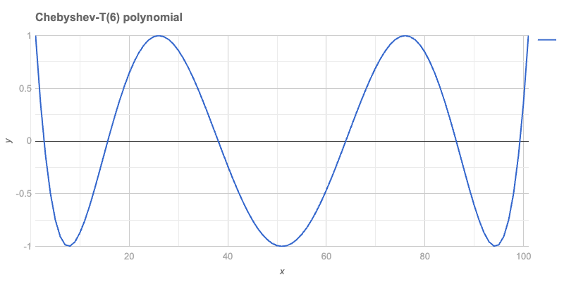

Basis

In fitting, bases of functions are crucial. The first eight Chebyshev-T polynomials are plotted to illustrate this.

my $n = 8;
my @data = (-1, -0.98 ... 1).map: -> $x {
    [x => $x, |(0..$n).map({
         .Str => chebyshev-t($_, $x, :$method)
     })].Hash
}

deduce-type(@data):tally;

# Tuple([Struct([0, 1, 2, 3, 4, 5, 6, 7, 8, x], [Num, Num, Num, Num, Num, Num, Num, Num, Num, Int]) => 1, Struct([0, 1, 2, 3, 4, 5, 6, 7, 8, x], [Num, Num, Num, Num, Num, Num, Num, Num, Num, Rat]) => 100], 101)

The plot with all eight functions is shown below:

#%html
js-google-charts('LineChart', @data,
    column-names => ['x', |(0..$n)».Str],
    title => "Chebyshev T polynomials, 0 .. $n",
    :$titleTextStyle,
    width => 800, 
    height => 400,
    :$backgroundColor, :$hAxis, :$vAxis,
    legend => merge-hash($legend, %(position => 'right')),
    chartArea => merge-hash($chartArea, %(right => 100)),
    format => 'html', 
    div-id => "cheb$n",
    :$format,
    :png-button)

Text Plot

Text plots provide a reliable method for visualizing data anywhere! The data is converted into a long form to facilitate plotting using “Text::Plot”.

my @dataLong = to-long-format(@data, <x>).sort(*<Variable x>);
deduce-type(@dataLong):tally

# Tuple([Struct([Value, Variable, x], [Num, Str, Int]) => 9, Struct([Value, Variable, x], [Num, Str, Rat]) => 900], 909)

A sample of the data is provided:

@dataLong.pick(8)
  ==> {.sort(*<Variable x>)}()
  ==> to-html(field-names => <Variable x Value>)

Variable	x	Value
1	-0.18	-0.18
3	-0.44	0.979264
3	0.66	-0.830016
6	-0.92	-0.7483020369919988
6	0.56	0.9111532625919998
8	-0.6	0.42197247999999865
8	0.08	0.8016867058843643
8	0.66	0.8694861561561088

The text plot is presented here:

my @chebInds = 1, 2, 3, 4;
my @dataLong3 = @dataLong.grep({
    $_<Variable>.Int ∈ @chebInds
}).classify(*<Variable>).map({
    .key => .value.map(*<x Value>).Array
}).sort(*.key)».value;

text-list-plot(@dataLong3,
  width => 100,
  height => 25,
  title => "Chebyshev T polynomials, 0 .. $n",
  x-label => (@chebInds >>~>> ' : ' Z~ <* □ ▽ ❍>).join(', ')
);

# Chebyshev T polynomials, 0 .. 8                                   
# +----+---------------------+---------------------+---------------------+---------------------+-----+      
# |                                                                                                  |      
# +    ❍                  ▽▽▽▽▽▽▽▽               ❍❍❍❍❍❍                                       *❍     +  1.00
# |     □              ▽▽▽        ▽▽▽         ❍❍❍      ❍❍❍                               ***** □     |      
# |      □□          ▽▽              ▽▽     ❍❍            ❍                          ****    □□▽     |      
# |     ❍  □        ▽▽                 ▽▽▽ ❍               ❍❍                   *****       □ ▽❍     |      
# |         □      ▽                     ❍❍▽                 ❍❍             *****          □         |      
# +          □□   ▽                     ❍  ▽▽                  ❍        ****             □□  ▽       +  0.50
# |      ❍    □  ▽                     ❍     ▽                  ❍  *****                □   ▽ ❍      |      
# |            ▽▽                    ❍❍       ▽▽               **❍*                    □             |      
# |       ❍      □□                 ❍           ▽▽        *****   ❍                  □□    ▽ ❍       |      
# |           ▽    □                ❍             ▽▽  *****        ❍                □     ▽          |      
# +        ❍  ▽     □□             ❍              *▽**              ❍             □□     ▽  ❍        +  0.00
# |          ▽       □□           ❍          *****  ▽▽               ❍          □□                   |      
# |         ❍          □□        ❍       ****         ▽▽              ❍        □□       ▽  ❍         |      
# |                      □□    ❍❍   *****               ▽              ❍❍    □□        ▽             |      
# |        ▽ ❍             □□ ❍ *****                    ▽▽              ❍ □□         ▽▽  ❍          |      
# +       ▽   ❍             *❍□*                          ▽▽             ❍□          ▽   ❍           + -0.50
# |                    ***** ❍ □□□                          ▽▽        □□□ ❍         ▽                |      
# |      ▽    ❍    ****    ❍❍     □□□                         ▽▽   □□□     ❍❍     ▽▽    ❍            |      
# |     ▽     *❍❍**      ❍❍         □□□□                        ▽▽□          ❍❍ ▽▽     ❍             |      
# |       *****  ❍     ❍❍               □□□□□             □□□□□□  ▽▽▽▽        ▽❍❍     ❍              |      
# +    ▽**        ❍❍❍❍❍                      □□□□□□□□□□□□□□           ▽▽▽▽▽▽▽▽  ❍❍❍❍❍❍               + -1.00
# |                                                                                                  |      
# +----+---------------------+---------------------+---------------------+---------------------+-----+      
#      -1.00                 -0.50                 0.00                  0.50                  1.00         
#                                      1 : *, 2 : □, 3 : ▽, 4 : ❍

Fitting

This section presents the generation of “measurements data” with noise and the fitting process using a function basis.

my @temptimelist = 0.1, 0.2 ... 20;
my @tempvaluelist = @temptimelist.map({
    sin($_) / $_
}) Z+ (1..200).map({
    (3.rand - 1.5) * 0.02
});
my @data1 = @temptimelist Z @tempvaluelist;
@data1 = @data1.deepmap({ .Num });

deduce-type(@data1)

# Vector(Vector(Atom((Numeric)), 2), 200)

Rescaling of x-coordinates is performed as follows:

my @data2 = @data1.map({ my @a = $_.clone; @a[0] = @a[0] / max(@temptimelist); @a });

deduce-type(@data2)

# Vector(Vector(Atom((Numeric)), 2), 200)

A summary of the data is provided:

sink records-summary(@data2)

# +------------------+----------------------------------+
# | 0                | 1                                |
# +------------------+----------------------------------+
# | Min    => 0.005  | Min    => -0.23878758770507946   |
# | 1st-Qu => 0.2525 | 1st-Qu => -0.053476022454404415  |
# | Mean   => 0.5025 | Mean   => 0.07323149609113122    |
# | Median => 0.5025 | Median => -0.0025316517415275193 |
# | 3rd-Qu => 0.7525 | 3rd-Qu => 0.07666085422352723    |
# | Max    => 1      | Max    => 1.0071290191857256     |
# +------------------+----------------------------------+

The data is plotted below:

#% html
js-google-charts("Scatter", @data2, 
    title => 'Measurements data with noise',
    :$backgroundColor, :$hAxis, :$vAxis,
    :$titleTextStyle, :$chartArea,
    width => 800, 
    div-id => 'data', :$format,
    :png-button)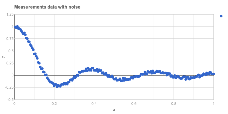

A function to rescale from [0,1] to [-1, 1] is defined:

my &rescale = { ($_ - 0.5) * 2 };

The basis functions are listed:

my @basis = (^16).map: { chebyshev-t($_) o &rescale }
@basis.elems

# 16

Remark: The function composition operator o is utilized above. The argument is rescaled before computing the Chebyshev polynomial value.

A linear model fit is computed using these functions:

my &lm = linear-model-fit(@data2, :@basis)

# Math::Fitting::FittedModel(type => linear, data => (200, 2), response-index => 1, basis => 16)

The best fit parameters are:

&lm('BestFitParameters')

# [0.18012514065989924 -0.3439467053791086 0.29469719162086117 -0.20515007850826206 0.12074121627488964 -0.003435776130307378 -0.047297896072549465 0.08663571434303828 -0.058165484141402886 -0.03933300920226471 0.03907623399167609 0.0015109810557268964 -0.011525135506292928 -0.0045136819929066 0.0021477767328720826 -0.004624145810439574]

The plot of these parameters is shown:

#% html
js-google-charts("Bar", &lm('BestFitParameters'), 
    :!horizontal,
    title => 'Best fit parameters',
    :$backgroundColor, 
    hAxis => merge-hash($hAxis, {title => 'Basis function index'}), 
    vAxis => merge-hash($hAxis, {title => 'Coefficient'}), 
    :``titleTextStyle, :``chartArea,
    width => 800, 
    div-id => 'bestFitParams', :$format,
    :png-button)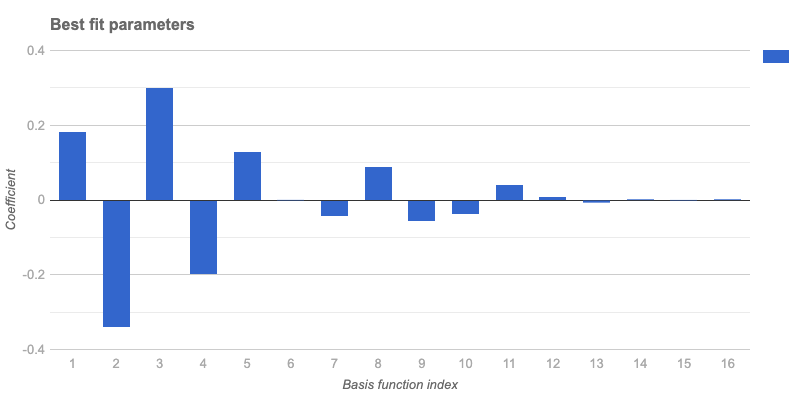

It is observed from the plot that using more than 12 basis functions does not improve the fit, as coefficients beyond the 12th index are very small.

The data and the fit are plotted after preparing the plot data:

my @fit = @data2.map(*.head)».&lm;
my @plotData = transpose([@data2.map(*.head).Array, @data2.map(*.tail).Array, @fit]);
@plotData = @plotData.map({ <x data fit>.Array Z=> $_.Array })».Hash;

deduce-type(@plotData)

# Vector(Assoc(Atom((Str)), Atom((Numeric)), 3), 200)

The plot is presented here:

#% html
js-google-charts('ComboChart', 
    @plotData, 
    title => 'Data and fit',
    column-names => <x data fit>,
    :``backgroundColor, :``titleTextStyle :``hAxis, :``vAxis,
    seriesType => 'scatter',
    series => {
        0 => {type => 'scatter', pointSize => 2, opacity => 0.1, color => 'Gray'},
        1 => {type => 'line'}
    },
    legend => merge-hash($legend, %(position => 'bottom')),
    :$chartArea,
    width => 800, 
    div-id => 'fit1', :$format,
    :png-button)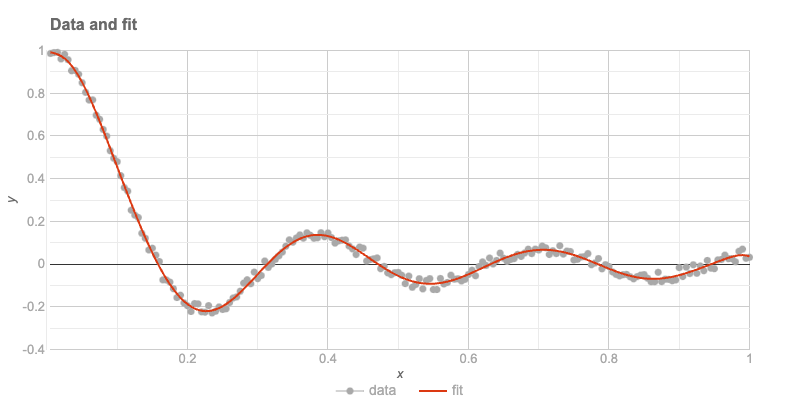

The residuals of the last fit are computed:

sink records-summary( (@fit <<->> @data2.map(*.tail))».abs )

# +----------------------------------+
# | numerical                        |
# +----------------------------------+
# | Max    => 0.03470224056776856    |
# | Median => 0.0136727625440904     |
# | Min    => 0.00011187750898611348 |
# | 1st-Qu => 0.006365201141942046   |
# | Mean   => 0.01363628423382272    |
# | 3rd-Qu => 0.019937969354319008   |
# +----------------------------------+

Condition Number

The Ordinary Least Squares (OLS) fit is computed using the formula:

β=(t(X).X)^(-1).t(X).y, where t(X) is the transpose of X.

The condition number of the “normal matrix” (or “Gram matrix”) t(X).X is examined. The design matrix is obtained first:

my @a = &lm.design-matrix();
my $X = Math::Matrix.new(@a);
$X.size

# (200 16)

The Gram matrix is:

my $g = $X.transposed.dot-product($X);
$g.size

# (16 16)

The condition number of this matrix is:

$g.condition

# 88.55110861577737

It is concluded that the design matrix is suitable for use.

Remark: For a system of linear equations in matrix form Ax＝b, the condition number of A, k(A), is defined as the maximum ratio of the relative error in x to the relative error in b.

Remark: Typically, if the condition number is k(A)=10^d, up to d digits of accuracy may be lost in addition to any loss caused by the numerical method (due to precision issues in arithmetic calculations).

Remark: A very “Raku-way” to define an ill-conditioned matrix is as “almost not of full rank” or “almost as if its inverse does not exist.”

Temperature Data

The entire workflow is repeated with real-life data, specifically weather temperature data for four consecutive years in Greenville, South Carolina, USA. This location is where the Perl and Raku Conference 2025 will be held.

The time series data is ingested:

my $url = 'https://raw.githubusercontent.com/antononcube/RakuForPrediction-blog/refs/heads/main/Data/dsTemperature-Greenville-SC-USA.csv';

my @dsTemperature = data-import($url, headers => 'auto');
@dsTemperature = @dsTemperature.deepmap({ ``_ ~~ / ^ \d+ '-' / ?? DateTime.new(``_) !! $_.Num });
deduce-type(@dsTemperature)

# Vector(Struct([AbsoluteTime, Date, Temperature], [Num, DateTime, Num]), 1462)

A summary of the data is shown:

sink records-summary(
  @dsTemperature, field-names => <Date AbsoluteTime Temperature>
);

# +--------------------------------+----------------------+------------------------------+
# | Date                           | AbsoluteTime         | Temperature                  |
# +--------------------------------+----------------------+------------------------------+
# | Min    => 2018-01-01T00:00:37Z | Min    => 3723753600 | Min    => -5.72              |
# | 1st-Qu => 2019-01-01T00:00:37Z | 1st-Qu => 3755289600 | 1st-Qu => 10.5               |
# | Mean   => 2020-01-01T12:00:37Z | Mean   => 3786868800 | Mean   => 17.053549931600518 |
# | Median => 2020-01-01T12:00:37Z | Median => 3786868800 | Median => 17.94              |
# | 3rd-Qu => 2021-01-01T00:00:37Z | 3rd-Qu => 3818448000 | 3rd-Qu => 24.11              |
# | Max    => 2022-01-01T00:00:37Z | Max    => 3849984000 | Max    => 29.89              |
# +--------------------------------+----------------------+------------------------------+

The plot of the data is provided:

#% html
js-google-charts("Scatter", @dsTemperature.map(*<Date Temperature>), 
    title => 'Temperature of Greenville, SC, USA',
    :$backgroundColor,
    hAxis => merge-hash($hAxis, {title => 'Time', format => 'M/yy'}), 
    vAxis => merge-hash($hAxis, {title => 'Temperature, ℃'}), 
    :``titleTextStyle, :``chartArea,
    width => 1200, 
    height => 400, 
    div-id => 'tempData', :$format,
    :png-button)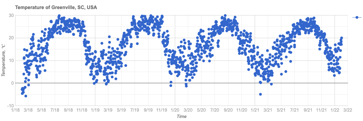

The fit is performed with rescaling:

my (``min, ``max) = @dsTemperature.map(*<AbsoluteTime>).Array.&{
  (.min, .max)
}();

# (3723753600 3849984000)

my &rescale-time = {
    -(``max + ``min) / (``max - ``min) + (2 * ``_) / (``max - $min)
}
my @basis = (^16).map({ chebyshev-t($_) o &rescale-time });
@basis.elems

# 16

my &lm-temp = linear-model-fit(
  @dsTemperature.map(*<AbsoluteTime Temperature>), :@basis
);

# Math::Fitting::FittedModel(type => linear, data => (1462, 2), response-index => 1, basis => 16)

The plot of the time series and the fit is presented:

my @fit = @dsTemperature.map(*<AbsoluteTime>)».&lm-temp;
my @plotData = transpose([
  @dsTemperature.map(*<AbsoluteTime>).Array,
  @dsTemperature.map(*<Temperature>).Array,
  @fit
]);
@plotData = @plotData.map({ <x data fit>.Array Z=> $_.Array })».Hash;

deduce-type(@plotData)

# Vector(Assoc(Atom((Str)), Atom((Numeric)), 3), 1462)

#% html

my @ticks = @dsTemperature.map({
    %( v => ``_<AbsoluteTime>, f => ``_<Date>.Str.substr(^7))
})».Hash[0, 120 ... *];

js-google-charts('ComboChart', 
    @plotData,
    title => 'Temperature data and Least Squares fit',
    column-names => <x data fit>,
    :``backgroundColor, :``titleTextStyle,
    hAxis => merge-hash($hAxis, {title => 'Time', :@ticks, textPosition => 'in'}), 
    vAxis => merge-hash($hAxis, {title => 'Temperature, ℃'}), 
    seriesType => 'scatter',
    series => {
        0 => {type => 'scatter', pointSize => 3, opacity => 0.1, color => 'Gray'},
        1 => {type => 'line', lineWidth => 4}
    },
    legend => merge-hash($legend, %(position => 'bottom')),
    :$chartArea,
    width => 1200, 
    height => 400, 
    div-id => 'tempDataFit', :$format,
    :png-button)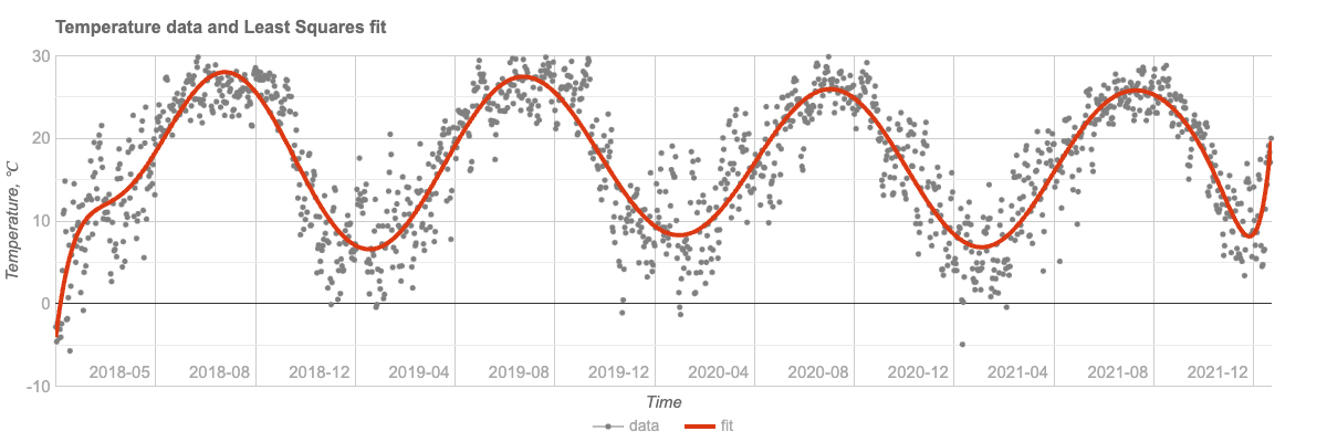

Future Plans

The current capabilities of Raku in performing regression analysis for both educational and practical purposes have been demonstrated.

Future plans include implementing computational frameworks for Quantile Regression in Raku. Additionally, the workflow code in this post can be generated using Large Language Models (LLMs), which will be explored soon.

5 thoughts on “Day 17 – Chebyshev Polynomials and Fitting Workflows”

Pingback: 2024.52 Connecting the Dots – Rakudo Weekly News
Anonymous says:

December 24, 2024 at 4:28 pm

In years past I used to use Legendre polynoials for fitting to data. This post has a lot of raku idioms to absorb, and some ideas that are new to me about fitting functions to data – thanx for this.

LikeLike

1. Anton Antonov Antonov says:
  
  December 25, 2024 at 4:35 pm
  
  Thank you for your interest! If you interested in reproducing the results of this post you can use the notebook.
  
  Also, currently the fitting code examples works much faster with this clone of “Math::Matrix”. (I will issue a review and a PR requests soon.)
  
  LikeLike
  
Pingback: The 2024 Raku Advent Posts – Raku Advent Calendar
Pingback: Day 2- Doing Data Science with Raku – Raku Advent Calendar

Day 17 – Chebyshev Polynomials and Fitting Workflows

Introduction

TL;DR

Setup

Why use Chebyshev polynomials in fitting?

Chebyshev polynomials computation

Computation Granularity

Precision

Plots

Single Polynomial

Basis

Text Plot

Fitting

Condition Number

Temperature Data

Future Plans

Published by Anton Antonov Antonov

5 thoughts on “Day 17 – Chebyshev Polynomials and Fitting Workflows”

Leave a comment Cancel reply

Introduction

TL;DR

Setup

Why use Chebyshev polynomials in fitting?

Chebyshev polynomials computation

Computation Granularity

Precision

Plots

Single Polynomial

Basis

Text Plot

Fitting

Condition Number

Temperature Data

Future Plans

Share this:

Related

Published by Anton Antonov Antonov

5 thoughts on “Day 17 – Chebyshev Polynomials and Fitting Workflows”

Leave a comment Cancel reply